6.3. Making a Seed Model Manually in 3dmod
The first step is to set up a seed model. Press Seed Fiducial Model Using 3dmod to open the prealigned stack and an empty model in 3dmod. The Bead Fixer module will also open in a mode that has features to help with the seeding process. These features are:
- Autocenter, which is turned on by default in this mode. This will allow you to position the cursor near a bead and add a point; the program will place the point on the center of gravity of the bead. For beads lighter than background, select Light.
- Automatic new contour, which makes a new contour when you pick a new bead. This is helpful because each bead must be in a separate contour; Beadtrack will try to extend each contour through the tilt series. Once you turn this option on, it will stay on between Bead Fixer sessions.
- Overlay, which displays the view being seeded and a nearby view in magenta-green overlay. This feature is intended to help you pick a good distribution of beads when they are on two surfaces. In the overlay, each bead will show up in magenta on the view being seeded and in green on the nearby view; the green will appear to the left or the right depending on which surface the bead is on. Click near the bead in magenta to add it. If you use reversed contrast to make the beads show up more clearly, the bead on the current view will still appear in magenta.
Pick a view near zero tilt that has good images of the beads. Put one point in the center of each desired bead. Beads too close to the edges are not trackable by Beadtrack but could be tracked by hand if necessary. Try to have at least 8 beads well distributed over the area, and well distributed between the two sides if they are on two surfaces. The more beads you have, the better the alignment will be, up to a point, but the more work it may take for you to complete the model. If the beads are all on one surface, there is not much point in having more than 12 or so; if they are on both surfaces, 20 or more may be useful. However, for areas larger than 1000x1000 pixels, you will probably need to use local alignments, in which case you should have at least 8-12 fiducials per 1000 by 1000 pixel area. (See Using Local Alignments.) Save the seed model when you are done.
6.4. Tracking Gold from a Seed Model
Beadtrack proceeds from one view to the next, tracking as many beads as possible on the new view. Once it has bead positions on enough views, it runs a simplified tilt alignment to get improved predictions of where beads should be and to reject erroneous positions. This procedure usually works well on small data sets, but may perform poorly when the data included in the tilt alignment do not give a good fit. The data can fit poorly when they are from a large area or when the tilt series includes very high angles. To address this problem, Beadtrack provides two ways to restrict the data so it fits the alignment better: 1) the tracking can be done over a series of overlapping subareas, so that the fit to the data is similar to that available when using local alignments; and 2) the number of views included in the tilt alignment can be restricted, so that high angle data from both ends of the tilt series are not included in the same fits. For particularly difficult data, both methods can be used.
Most standard entries to Beadtrack should work well, so in Basic mode Etomo shows only a few of the many parameters.
- View skip list Enter or adjust the list of views to be skipped over. If you put entries into the Exclude views field in the Etomo Setup window, these values will be carried over to this box. Skip over a view if there is a big mag change for that view only, or a particularly poor image for that view. Typically you would leave this entry blank on a first run and enter a view number here for a second run if the program fails to track accurately through that view.
- Separate view groups Specify one or more lists of views that should be kept out of groupings with adjacent views. If your data might have a sudden lurch in magnification or tilt angle, entering a separate view group will avoid having views on both sides of this discontinuity assigned the same value for such variables. Taking a tilt series in two directions instead of all in one direction introduces such a discontinuity; you should always identify such tilt series during the tomogram setup so that a separate view group will be defined for you (see the section on bidirectional tilt series). In cases of discontinuity, you would list all the views up to the discontinuity (or all of the views after it). More rarely, there might be views that don't match the surrounding ones for some other reason. Enter a list with no embedded spaces, and use a space to separate multiple lists.
- Refine center with Sobel filter should be turned on because it will almost always give more precise centering of the model points on the beads. (When it does not, the program falls back to the positions found using the centroids of the beads.) Using this method typically reduces the mean residual for fine alignment by ~22% for plastic section data sets and ~10% for cryo data sets, provided that the alignment is intrinsically good and not dominated by systematic misfit. However, it can be detrimental for a cryo data set unless the Sobel sigma relative to bead size is set to about 0.12; thus the option is not on by default. Selecting one of the system templates during tomogram setup will turn on the option and supply the appropriate filtering parameter.
- Overall low-pass filter cutoff should be set for particularly noisy images, such as cryo data with a small pixel size in the coarse aligned stack. The entry is in reciprocal nanometers to allow using a value that is nearly insensitive to binning and pixel size. Optimal values have been found to be in the range of 0.3-0.4/nm for typical cryo data with a range of pixel sizes and binnings. The same filter is applied at all tilt angles; tests indicated no value in having a variable filter such as would be obtained by applying dose-weighting to a dose-symmetric series.
- If you have partially tracked a bead in the seed model and left a gap because of ambiguity, you should uncheck Fill seed model gaps.
- Local tracking With this option on, the program does tracking in overlapping, local subareas. When it is selected, you can change the value in the Local area size text box, which specifies a target size for the local areas. The default size is rather large and smaller values may give better results in some cases. As of IMOD 4.7, this option is on by default.
- Max # of views to include in align Put a value in this text box to make the tilt alignments fit to data from a restricted range of views. Try a value equal to half the number of views in the series.
- If you have finer than 1 degree tilts, you may need to increase the Minimum # of views for tilt alignment (in Advanced).
Press Track Seed Model. Open the track.log file and skip to the end to see a summary of which beads could not be tracked completely. If several beads fail to track past a particular view, you might want to add that view to the list of views to be skipped and rerun the tracking.
Next press Fix Fiducial Model to read the new fiducial model into 3dmod. The Bead Fixer dialog box will appear in the gap-filling mode. It will allow you to jump from one gap in the data to the next and fill in missing points if appropriate. It is acceptable for some of the points to be missing on some of the views. If too few of the points can be extended all the way to the first or last views, you can add some fiducials that are present only in higher tilt views. Just be sure to add them on a substantial number of views, not just on a few, so that their 3-D positions can be solved for accurately. If you do need to add several fiducials, you could put some "seeds" into your edited fiducial model and allow Beadtrack to track those beads as far as possible.
6.5. Using Beadtrack to Extend a Model
Sometimes you will want to have Beadtrack start with an existing fiducial model instead of a seed model. This is especially helpful when there are a large number of beads that failed to track. For example, you might extend some fiducials past a view where they failed to track then try to get Beadtrack to track them the rest of the way, or you might want to add fiducials when you realize that you need to use local alignments. To use the existing fiducial model as a seed for another run, press Track with Fiducial Model as Seed. Your original seed model will be renamed to "setname_orig.seed" the first time that you do this. Then press Fix Fiducial Model to read the retracked model into 3dmod. You can repeat this operation as many times as needed. This procedure will tend to fill in gaps in the model, which is usually appropriate. However, if you have already left some gaps in the model because of ambiguities, you should uncheck Fill seed model gaps.
6.6. Getting Fiducials for a Second Axis
For a double-tilt series, there are two methods for getting an initial alignment of the reconstructions: from the positions of fiducial markers that match between the two series, or by cross-correlations of the two volumes (new in IMOD 4.9). An alignment based on fiducials is much quicker and somewhat more reliable, especially if there is substantial warping between the volumes, so it is the preferred method when there are enough fiducials. It requires that at least some (8-10) of the beads be the same in the two series. The script Transferfid will help ensure this by making a seed model for the second axis based on the fiducial model for the first axis. To use this tool, complete your fiducial model for the first axis. Proceed through the coarse alignment steps for the second axis until you reach the Fiducial Model Generation panel. If your tilt angles are not in ".rawtlt" files, you also must fill in the view numbers of the zero-tilt views in the Center view text boxes (visible in Advanced mode). Press Transfer Fiducials from Other Axis to begin the operation. Transferfid will search for the pair of views in the two series that correspond the best, then transfer the fiducials from the first series to make the seed model for the second series. At the end, the program indicates the number of fiducials that failed to transfer and how the contour numbers correspond between the first fiducial model and the new seed model. This information is saved in a transferfid.log file. Transferfid also creates a file called "transferfid.coord" with the information needed for the first stage of the tomogram combining procedure to determine how fiducials correspond between the two tilt series. As long as this information is available, you can add and delete fiducials from either tilt series after doing the transfer, and the combining procedure will still be able to tell which fiducials correspond.
When there is a substantial shift between the areas captured in the two axes, the transferred fiducials will not cover the area for the second axis. If you used automatic seed selection successfully on the first axis, you can use it again to add fiducials in the remaining area. Simply switch to Generate seed model automatically, set appropriate parameters, and press Generate Seed Model to add points to the model.
Transferfid can fail, although it is more robust in IMOD 4.9 because it can handle deviations from 90 degree rotation of up to ~25 degrees and it can automatically detect when images are mirrored with respect to each. (Mirroring occurs when the sample was turned upside-down between the series.) If Transferfid does fail to work, as indicated by an unusually large number of fiducials that failed to transfer or a seed model that contains incorrect model points, you may need to set the translational and rotational alignment between the two series manually with Midas. To do this, just check Run midas and run the transfer again. Midas will start up with the center views from the two tilt series. Adjust the alignment with translation and rotation (left and middle mouse buttons). Do not be alarmed if you have to rotate the image by 180 degrees, just select Interpolate to get a good rotated image. If the images cannot be aligned because the sample was inverted, select "Mirror around X-axis" from the Edit menu and then align the images. Save the transformation and exit. The search for the best corresponding pair of views will proceed using this starting alignment.
In Advanced mode, you can specify the views to search around and limit or expand the number of views in the search. As a last resort, you could set the Number of views in the search to 1 and set the alignment as well as possible in Midas, including a magnification change and stretch.
If the transfer operation still fails, it would be possible to add seed points by hand in the second axis in the same order that they occur in the first axis, but it is probably much more convenient to plan on using the volume alignment by cross-correlation when you combine the volumes. If you want to generate the seed model automatically, be sure to uncheck Add beads to existing model first.
6.7. Local Patch Tracking
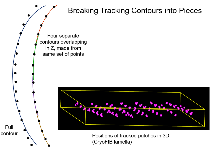
When there are insufficient fiducials, local patch tracking can provide a significantly better alignment than the basic correlation alignment. Patch tracking starts out with a set of overlapping patchs of image at zero tilt. For each patch, it aligns a comparable patch at the next tilt and places a model point at the center of the aligned patch. This process continues for each patch, aligning a patch at each tilt to the patch at the previous tilt. A contour in the resulting model represents the behavior of the whole image patch, not the location of any particular feature in the patch. Over long extents of tilt this kind of correlation is just as vulnerable as whole-image correlations to having the features dominating the correlation change and shift, but having many patches that can behave differently may reduce the consequences of such changes. Patch tracking allows an alignment that includes a solution for the tilt axis angle and that can correct for shrinkage or magnification changes. Even if there are fiducials, the patch tracking may provide a tomogram of adequate quality in some cases, so it may be worth trying as a way to reduce labor.
One feature that requires some extended explanation is the option to break
contours into overlapping pieces. Normally the positions from tracking each
patch are placed into a single contour, just as for real fiducials. The mean
residual from a fine alignment with such contours will be directly comparable
to the mean residual from a regular fiducial alignment. A high value
generally indicates that some or all of the patch positions do not track a
single 3D position in the specimen, which means the alignment is not globally
consistent. This happens because tracking a small patch by correlation is
susceptible to the same kind of progressive shifts in 3D position as occur
with an overall coarse alignment only by correlation. The option to break
contours into pieces provides a way to compensate partially for this problem.
The positions for each patch will be subdivided into a series of overlapping
contours, where the length of each contour is as specified, and the contours
overlap (contain identical points) over a certain number of views, 4 by
default. This is illustrated below on the left, where the points depict
tracked patch positions that would be seen in a view of the model looking along the
tilt axis, with a large Z-scale to spread out the points. The lines represent
the trajectory implied by the alignment solution. On the left, a solution
forced to fit all the points may deviate considerably from the points at the
ends and in the middle of the tilt range. On the right, fitting separately to subsets of
points allows the solution to fit much better within each range. The 3D model
on the right shows a typical case where the different subsets of points each
result in a different 3D position for the patch.
Breaking contours into pieces will have the following effects:
- The measures of alignment error will be reduced dramatically, from a combination of two factors. One factor is the change in average 3D position of the structure being tracked in the patch as the tilt changes, as illustrated above. The other factor is an improvement intrinsic to fitting the alignment equations over a smaller tilt range. The section below, Aligning with a Patch Tracking Model, provides estimates of the magnitude of the latter factor, which should help you interpret the changes in error. In general, the errors may go down by 20-40% without there being any actual improvement in alignment.
- The actual quality of the alignment may or may not be any better than that from fitting to whole contours, if you continue to fit to all of the patches. If the average 3D position of the material dominating the correlation between successive patches shifts through the series, the alignment should be better because it can more accurately solve for this shifting average position, instead of being forced to assume that the patch represents the same 3D position through the series.
- Even if the 3D patch positions are constant, breaking the contours into pieces makes it possible to identify segments that give the worst fit and eliminate them. Eliminating contours that are least consistent with a global alignment should improve the quality of alignment. The Bead Fixer has a special mode that allows you to find and remove contours with the largest mean residuals in the alignment. Moreover, with robust fitting during fine alignment, you can choose to have it use a single weight for all the points in a contour, and this will eliminate or give reduced weight to the worst-fitting contours.
Because contours broken into pieces give a misleadingly low mean residual, it is recommended that you first run tracking without breaking contours into pieces, then assess the alignment. If necessary, then go back and break contours into pieces. There is no need to recompute the patch correlations; just press the Recut or Restore Contours button to have the whole contours from the tracking broken into pieces according to the current parameters. Prior experience with similar data sets would allow you to skip the initial fitting and specify breaking into pieces when trackingthe patches.
A different iterative step will involve new patch correlations. If the fine alignment indicates that the specimen is tilted by more than a few degrees and requires a tilt angle offset to be level in the X/Z plane, it is recommended that the patch tracking be redone with that tilt angle offset. Both the cosine stretching used to match up successive patches at high tilt and the adjustment in measured shift to account for tilt will then be more accurate, potentially reducing the systematic errors when tracking.
Patch tracking is controlled by the following settings:
- Size of patches: You should choose a size based on the amount of image detail and the signal-to-noise ratio of the images. For stained plastic sections rich in image detail, patches can be in the range of 100-200 pixels. For frozen-hydrated material, patches will need to be much bigger, 500-1000 pixels. Cryo-sections might have enough image detail to allow patches at the lower end of this range; plunge-frozen material with sparse image data might require the largest patches.
- Number or overlap of patches: The number of patches can be controlled by the amount of overlap between adjacent patches. If you have large patches where the default overlap might give fewer patches than desired, you control the number of patches directly by selecting and specifying the Number of patches.
- Using a Boundary Model: If portions of the image do not have enough features to give good correlations, then you should exclude them by drawing one or more contours around regions that are suitable for correlation. Select Use Boundary Model, press Create Boundary Model, and pick a view at or near zero tilt on which to draw the boundary. Enclose one or more regions on this view. There is no need to draw contours on other views.
- Iterations to increase subpixel accuracy: When two images are correlated, the shift between them is estimated with subpixel accuracy by fitting parabolas to the correlation peak in X and Y. If the shift is then applied before repeating the correlation, the peak will become centered on a pixel and the inaccuracy of interpolation is reduced or eliminated. This might lead to an improvement in the final alignment, but in our experience so far the effect is slight. If you want to use this feature, try tracking with and without iterations to see how much it affects the residual of the alignment. Three iterations suffice to reduce the interpolation, but calculations will take 3 times as long.
- Breaking contours into pieces This option is discussed above. After enabling the option, you can adjust the length of pieces if desired. The default length is based on the number of views in the tilt series. You can also adjust the overlap between the pieces. Note that this is a minimum overlap; the overlap will usually be bigger than the minimum so that the contours can all have the specified length.
- Tilt angle Offset: (in Advanced mode) Enter the total angle offset suggested in the alignment log to use more accurate angles when correlating.
- Trimming area to analyze The Pixels to trim and the Min and Max entries for X and Y provide an alternative to using a boundary model for restricting the area to analyze. It is no longer necessary to set these limits in order to avoid correlating with portions of the prealigned stack that contain no image data (are filled with gray). Tiltxcorr will use the transforms applied in building the coarse aligned stack to determine where the gray areas are. It will skip patches that have too little usable image data and, for other patches with gray area, it will taper the data down to the gray area to minimize correlation artifacts.
See Aligning with a Patch Tracking Model for details on what to do differently in the alignment step.
6.8. Using RAPTOR to Make a Fiducial Model
The RAPTOR program from Stanford is part of IMOD and the option to use this program is available, but only for the first axis of a dual-axis data set. Its centering of fiducials will generally be worse than when using Beadtrack, and it may have trouble finding beads over the whole image when some areas are much darker than others. See the RAPTOR man page for details on its operation. First decide whether to run it on the raw stack or the prealigned stack. The latter case allows tighter tolerances for some distance parameters and is usually more successful. Decide on the number of beads to find per view and enter that in the Number of beads to choose text field. The Unbinned bead diameter field should have a correct value based on the pixel size and actual bead size that you entered in Setup.
Press Run RAPTOR to run the program, which will create a model file "setname_raptor.fid". It can take on the order of an hour with many beads. When it is done, press Open RAPTOR Model in 3dmod to see the resulting model on the appropriate stack. If the result is acceptable, then press Use RAPTOR result as Fiducial Model to rename the model to the standard name for a fiducial model. At this point, you can press Fix Fiducial Model to open the model in 3dmod with the Bead Fixer in gap filling mode, and you can also use Track with Fiducial Model as Seed to track additional points in the model in the conventional way with Beadtrack.
7. FINE ALIGNMENT
The goal of the final alignment is to transform the images so that they represent projections of a solid body tilted around the Y axis, as well as to refine the projection angles. In order to transform the images, one needs to determine the rotation, translation, and scaling (magnification) to be applied to each image. It is also possible to solve for variables which will correct for linear distortions of the specimen.
7.1. Running Tiltalign
Whether you have fiducials on one surface or two determines what variables can be solved for. If there are beads on only one surface, you can solve for either tilt angles or stretch in the X direction but not both. If there are beads distributed through the depth of the sample (typically but not necessarily on two surfaces), you can solve for both tilt angles and distortion.
Before computing an alignment for the first time, check the following settings in the General parameter page:
- Separate view groups. Specify one or more lists of views that should be kept out of groupings with adjacent views. See the discussion of the corresponding entry to Beadtrack under Fiducial Model Generation .
- List of views to exclude. Add to or adjust the views to be excluded, if necessary, in this text box. Again, if you entered Views to exclude in the Etomo Setup window, they will be carried over to this box.
- Analysis of Surface Angles Change the selection from Assume fiducials on 2 surfaces for analysis to Do not sort fiducials into 2 surfaces for analysis if the beads are not located on two distinct surfaces. Note that this setting does not affect the actual global alignment solution, just the analysis of the orientation of the section surface in space, which is done after the alignment solution is obtained.
Press Compute Alignment and examine the results in the log file after the process is done. The lengthy log file has been split into useful sections under different tabs. The first page that you see, Errors, shows three useful summary values. One is the ratio of measured values to unknowns, which provides a rough indication of how robust the solution is against random errors and of whether there might be too many independent variables being solved for. The second is the residual error mean, a global measure of the quality of the fit. A residual error is the distance between the measured position of a fiducial on a view and the position predicted by the alignment solution. The distance is in nanometers, or in pixels if no pixel size is available.
The third value is the "leave-out" error, which is a much better measure of the quality of the fit and of whether too many variables are being solved for, as explained in the next section. This error is estimated by running the alignment with a small fraction of points left out, typically about 5%, then using the solution to predict the positions of the points left out. The leave-out error is the mean distance between predicted and actual positions for the points left out, averaged over enough runs with different points left out to give reasonably accurate estimates. This process is called cross-validation. These errors are estimated as long as Compute prediction errors for points left out of test fits is checked.
A good alignment has a mean residual error of 0.25 to 0.6 nm. Often it will require local alignments to achieve such a value, especially for tilt series from plastic sections.
You can view a model of the residuals at every point, exaggerated by a factor of 10, by pressing the View Residual Vectors button (see Residual Model Output). This feature is particularly useful for assessing whether you need to use local alignments.
The Solution page shows the value of some of the alignment variables for each view. Examine the tilt angles, looking for places where they change by unusual amounts. The column labeled "deltilt" shows the difference between the solved tilt angle and the original, nominal tilt angle. This column should change gradually when tilt angles are grouped. Tilt angles are grouped by default because low tilt angles cannot be solved for accurately without grouping (see below). The "mag" column shows the effect of overall shrinkage and slight magnification changes due to changes in focus. If the "mag" column shows a sudden change that is much larger than surrounding changes, consider making all of the views after this change be a separate view group, as described above. For the variables that are grouped, this will keep views on the two sides of the transition from being constrained to having the same or similar values.
The last column on the Solution page, "mean resid", shows the mean error (residual) in nanometers for all of the points on each particular view. This information will reveal whether some views give a poorer fit than others.
Plots of the various columns in the solution versus view number can be seen by right-clicking over the Alignment panel and selecting one of the "Plot" options from the popup menu.
The Surface Angles page shows the results of an analysis of the solved bead positions in 3D and recommends a change in tilt angles that would make the beads lie in a horizontal plane. For plastic sections with gold on one or two surfaces, or when using patch tracking, make the recommended change at least after the first run of Tiltalign by taking the value shown for "Total tilt angle change" on the last line and using it in the Total tilt angle offset text box. It is not necessary to do this repeatedly because the final tilt angle offset will be determined in a later processing step. For cryo-samples with fiducials, it can easily be inappropriate to make this change and it is probably safest to skip it. Before making the change, examine the 3D model of fiducials in the X/Z side view and use the solved offset only if all gold is on one surface, or if it is so well-distributed that a line fit to these points should represent the overall pitch of the specimen.
You can open the Large Residual page to see the list of fiducials with the largest errors (in pixels here), but it is easier to deal with this information from the Bead Fixer dialog in 3dmod, which is opened in big residual mode when you press View/Edit Fiducial Model. The Bead Fixer is told what log file to read, so you can proceed without pressing Open Tiltalign Log File. Examine the points in turn by pressing the Go to Next Big Residual button (or the apostrophe hot key), paying particular attention to ones with errors greater than 2 pixels. Adjust point positions in the model, if appropriate. When you want to recompute the alignment after fixing some points, you can press Save & Run Tiltalign, which will save the model, rerun Tiltalign, and read in the new log file. There is one trap to this convenience button: Bead Fixer has no way of knowing if you have changed parameters in Etomo, so when you do change alignment parameters, you must compute the alignment through the button in Etomo instead. The Bead Fixer will be told to reread the log file after the alignment is done.
In Bead Fixer there is a button to Move Point by Residual. This button will move a point to the position that fits the mathematical model from the alignment. The image data are not consulted with regard to this movement, and sometimes the movement is inappropriate. This button is there for convenience, but you should not use it if it moves a point away from the center of the gold bead. This will often be the case if you are going to need local alignments. An even more convenient and powerful button is Move All by Residual. As explained in Using Robust Fitting, it is preferable to use robust fitting to reduce the effects of erroneous points than to move points blindly by their residuals. If you do use this feature, you should not do so until you have gone through enough points one by one to be confident that it will not move points away from the beads. In addition, you should select Neighboring views in the Residual Reporting box so that the criterion for whether to consider a residual large will be based on the residuals of other points on nearby views. This will keep the points on the high tilt views from always being selected as having the highest residuals. Otherwise, you may end up misaligning the high tilt views in the data set by using this button.
In the align log, you can also open the Fiducial Coordinates page to see the 3D coordinates that have been solved for the fiducials, as well as the mean residual in the fit for each fiducial. It is easier to visualize these points in 3dmodv by pressing the View 3D Model button on the Fine Alignment panel. If you indicated that points are on two surfaces, then the points will be sorted into two objects based on which surface Tiltalign thought they were on. This is a good way to assess whether the points are well enough distributed on both surfaces to support solving for distortion, particularly when local alignments are to be used.
7.2. Background on Grouping Variables and Cross-Validation
Variables are grouped in order to reduce the number of variables being solved for. Instead of solving for a different tilt angle for each view, with grouping by 5 the program will solve for a tilt angle for every fifth view and determine the angle for the rest of the views from the ones that it is solving for. This reduces the number of tilt variables being solved for by a factor of 5, and also averages over a larger number of measurements when solving for each individual value. Because of this averaging out of random errors, grouping will actually give a more reliable solution for variables that are hard to solve for, such as tilt angle near zero degrees. It is for this reason that you should always use grouping of tilt angles even when you are not solving for distortion.
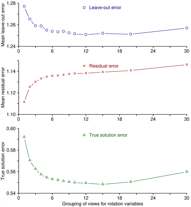
The way in which grouping prevents overfitting to random errors
can be demonstrated easily by considering the behavior of the leave-out error
versus the residual error as grouping is changed. Adding variables to the
solution (e.g., by adding a parameter or by reducing the grouping of an
existing parameter) will virtually always improve the mean residual simply because
there are more variables to adjust to fit the data. This is illustrated by
the middle panel in the figure below, which is based on synthesized fiducial
positions with random errors added. To obtain these curves, alignments were
run with a range of group sizes for rotation, and values were averaged over
multiple trials with
different random errors. The mean residual changes monotonically with
grouping. However, reduced grouping does not
necessarily give a better solution just because this error is less. The
ability of the solution to predict the actual positions is reflected more
accurately by the leave-out error, shown in the upper panel. As here,
leave-out error generally follows a U-shaped curve. As variables are added
(moving to the left in this graph), eventually a point is reached where
overfitting to the points that happen to be included makes the solution less
able to predict the positions of other points, and the leave-out error rises.
In the other direction,
fitting to fewer variables will eventually reach a point where there are too
few variables to account for the actual changes during the tilt series, and
the leave-out error again rises. In this case, because these are simulated
data, the true solution is known, and the deviation from the true solution is
plotted in the bottom curve. The minimum value for the leave-out error and
the minimum error from the true solution are reached at about the same grouping.
Thus, the leave-out error is a reliable indicator of whether the data are
being overfit or underfit.
You can easily see the same pattern in your own data by varying the settings for one variable. Since tilt angle is grouped by default, it is the most convenient to do this with. Run the alignment with the default Group size, with some smaller sizes, and with Solve for all except minimum tilt. The mean residual will decline, but you will most likely see the leave-out error increase at some point. If you increase group size, you should eventually see the leave-out error increase, unless tilt angle is best left out of the solution. This tedious process is automated by a script, Restrictalign, that assesses how leave-out error changes with increased grouping or elimination of each variable, then selects optimal settings that minimize this error.
In sum, whenever you change the variables being fit, use the leave-out error to assess whether the change is beneficial and ignore the mean residual. However, if you are improving the fiducial positions, both measures should drop and you can focus on the mean residual. For this reason, when "Save & Run Tiltalign" is used in the Bead Fixer window, the computation of leave-out error will be skipped to save time. After selecting all the alignment parameters that seem appropriate, use Restrictalign to minimize overfitting.
The reduction in number of variables by grouping becomes particularly important when you have a large number of fiducials (e.g., more than 150) or a large number of views (e.g., more than 140). In these cases, the program may have trouble finding a solution unless you also group some variables that are not grouped by default, namely rotation angle and magnification.
At the other end of the spectrum, when there are relatively few fiducials, grouping is important because it allows a variable to be included without inducing overfitting. In this case, use Restrictalign to select appropriate grouping or even eliminate variables automatically.
The grouping of variables can be done in two different ways. In one way, the particular parameter will change linearly from the first view in one group to the first view in the next group, and will appear to change smoothly over the whole tilt series. This is referred to as linear grouping or linear mapping. This method is used for every variable except stretch along the X-axis. For that variable, all of the views in a group will have exactly the same value.
Another point to be aware of is that some group sizes will vary with tilt angle. Group size for tilt angle will be proportional to the cosine of the angle, and will be set so that the average size equals the value that you specify for grouping. Because of the peculiar behavior of the X-axis stretch, its group size will change even more with tilt angle.
7.3. Background on Solving for Linear Distortion
The distortion solution is a strange beast. Even if the only thing happening to the section is a stretch along the X-axis, solving for distortion will successfully account for these changes, but the resulting solution will not numerically reproduce the amount of stretch. The problem is that there is an infinity of equivalent solutions, which all account for the distortion equally well, but differ in the geometry of the resulting reconstruction. This geometric difference is a "strain", a shifting in Z proportional to the X value of a column of pixels. Without additional information about the section, there is no way to recover its true structure, and the actual amount of stretching that occurred. The program needs to pick one solution out of the equivalent ones, and it does so by eliminating one variable; thus you will notice a variable listed as "dummy" in the Mappings page of the log file. Typically, this arbitrarily selected solution will change the most at high tilt angles, sometimes dramatically so, even though the actual changes in the section happen at a nearly constant rate through the series.
The distortion solution will also account for thinning when tilt angle is allowed to vary as well; However, this requires there to be a good distribution of fiducials in Z: either enough on both surfaces of a plastic section, or a substantial and well-distributed fraction of fiducials not located on one surface for a cryo-sample. The equations governing this situation dictate that the X-axis stretch change rapidly at the highest tilts, even if thinning occurs at a regular rate through the series. Thus, regardless of whether there is section distortion or thinning, or both, it is almost inevitable that the X-axis stretch will change most rapidly at high tilt.
Finally, be aware that including distortion can lead the program into inappropriate solutions, in which the tilt angle and the X-axis stretch covary excessively. This can occur when there are too few fiducials, too great an imbalance between the number of fiducials on the two surfaces, substantial random errors in the locations of the model points, or a ratio of measurements to unknowns that is too low. The potential remedies are to increase group sizes or to give up on solving for distortion. Unfortunately, cross-validation does not reliably reveal when distortion should be omitted because of a poor distribution of fiducials in Z, but it will indicate if its grouping needs to be increased because of inadequate signal-to-noise ratio or other such issues.
7.4. Solving for Distortion - Fiducials on Both Surfaces
To solve for distortion, open the Global Variables page of the Fine Alignment panel and select Full solution in the Distortion Solution Type section. This will automatically switch to some good default values if you have fiducials on both surfaces, namely a grouping of 5 for tilt angles (if they are not already grouped), 7 for the stretch variable, and 11 for the skew variable. Grouping is important when solving for distortion because it dramatically reduces the number of variables to be solved for, averages out random errors better, and gives a more robust solution. The typical range for group sizes would be:
- 3 - 10 for tilt angles.
- 5 - 10 for X-stretch.
- 7 - 15 for skew angle.
You might want to pick the low end of these ranges of group sizes if an alignment run reveals that one of the distortion variables changes especially quickly (but don't be fooled by big changes for pictures taken out of sequence). In any case, you should do cross-validation with Restrictalign to make sure that the group sizes are not too small.
The stretch variable ("dmag" in the Solution page of the log file) will typically range from 0.001 to 0.02 but can easily reach 0.05 at high tilts. If you get values larger than 0.05, or if you get changes in tilt angle ("deltilt") more than 2 degrees, you should increase the group size and see if the range of values decreases, particularly if you have only 3-5 fiducials on the surface with fewer fiducials. If the range decreases substantially, stick with the larger group size. You can also increase the grouping for skew and tilt angles to try to get a better-behaved solution. If a solution seems unreasonable, either abandon the attempt to solve for distortion, or solve for skew angle only, as described in a few paragraphs.
The skew is an angle in degrees and will typically range from 0 to 1 degrees. Values greater than about 0.2 degrees are worth correcting for, and a change of more than about 0.3 degrees from one group to the next would be a big change.
If you have discovered that there is some sudden change in alignment such that two views should not be grouped together, then the simplest thing to do is to specify a Separate view group on the General parameters page. For example, if there is sudden change between views 30 and 31, enter 1-30 in this text box; more than one separate group can be entered if they are separated by spaces.
A finer degree of control over grouping of an individual variable can be achieved by making an entry in the Non-default groupings text box that appears in Advanced mode for each variable. To use a non-default grouping, enter the starting and ending view number and the group size, separated by commas. For example, if the default grouping for X-stretch is 10, but you want smaller groups for the first and last 20 views of a 121-view tilt series, then enter "1,20,5 102,121,5". Separate different non-default groupings with spaces, as in the example. Before making such changes, run Restrictalign to get a better idea if it is appropriate; it is not set up to handle non-default groupings.
7.5. Solving for Distortion - Fiducials on Only One Surface
If you have fiducials on only one surface, or only a few fiducials on one surface, you can't properly solve for both tilt angle and distortion. If the section has thinned but not distorted, then allowing the tilt angles to vary will correct for the thinning. If the section has distorted but not thinned, then solving for distortion with fixed tilt angles is appropriate. In reality, both phenomena occur, and section sag can also make the tilt angles inaccurate, so that fixing them completely is likely to be problematic. The simplest and safest thing to do in this situation is not to solve for distortion, especially if you are able to do local alignments, but here is a procedure if you want to explore including the distortion solution.
- Select the full distortion solution, and set the grouping for tilt angles to a large number (~30). Compute an alignment and check the behavior of the solution for "dmag" and "deltilt". It is possible for tilt angle and stretch to compensate for each other and give an artifactual solution, so if you see relatively large values for both of these (e.g., greater than 2-3 degree tilt angle change and x-stretch greater than 0.05-0.1), don't trust the result. Instead, do one of the following:
- If skew is not significant (say, less than 0.25 degrees), then don't solve for distortion, and set the group size for tilt angles at 5 to provide a better solution at low tilt angles.
- If skew is significant, then select Fixed tilt angles and continue to solve for distortion, perhaps reducing the group size accordingly. If skew is no longer significant in this solution, abandon solving for distortion as in the previous step; i.e., return to solving for tilt angles with a group size of 5.
7.6. Using Robust Fitting
Robust fitting is an iterative method in which data
points with larger fitting errors are given less weight when finding a
solution. If there are sufficient data points (in our case, fiducial
positions), it can keep the solution from being contaminated by a small number
of aberrant points. The procedure is illustrated here:
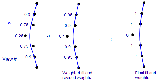
This is a side view of a few of the positions of one fiducial, where the
vertical axis is view number, the points show the X-coordinates of points in
the fiducial model, and the blue line is the X position predicted from the
solution fit to these data. In an ordinary fit (on the left), one bad point
tends to pull the fit away from the true positions of neighboring points.
When each point is given a weight that depends on its error (numbers to left),
the bad point gets the lowest weight. In a solution that minimizes a sum of
weighted errors (middle), the lower influence of the bad point reduces the
amount that it pulls the
solution away from true for the adjacent points. Their error decreases, the
bad point's error increases, and the weights change accordingly for the next
round. In an ideal case, iterating this procedure would reduce the weight of
the bad point to 0 (right). Realistically, clearly aberrant points might end
up with small non-zero weights, but still have very little effect on the
solution.
Select Do robust fitting with tuning factor on the General parameters page to activate robust fitting. The log file window will have a new Robust tab, showing the final mean weighted errors for global and local solutions, if any. The weighted errors will be less than with no robust fitting, but the unweighted error can actually be more because some down-weighted points will end up with larger errors. Leave-out errors are also shown with and without weighting. The best measure of whether the robust fitting is giving a better solution is the comparison of weighted leave-out errors, which is summarized by the last number on the line "Benefit from robust fitting". The tab will also show some details about the fitting, including a summary of how many points have final weights less than various thresholds. Typically, about 5% of points will have weights of 0.5 or less. You can enter a tuning factor less than 1 in the text box to downweight more points, or greater than 1 to downweight fewer points. The computed benefit will vary somewhat with this factor and can be used as a guide to whether a change is appropriate. Unfortunately, this benefit has turned out to be very small or negative for many data sets that have been tested.
The assignment of weights is done by statistical methods that are valid only with a certain minimum number of data points, so the robust fitting may fail if there are too few fiducials.
The advantage of robust fitting, in principle, is that it can suppress the effects of aberrant points and give essentially the same alignment solution that would be obtained if those points were shifted to the correct positions. Its properties should make it a better way to get an improved alignment than the questionable practice of blindly moving all points by their residuals in the Bead Fixer. Note in the figure above that moving the bad point by its residual in the original solution will not move it all the way to the correct location, and it can still contaminate the solution. After robust fitting, moving the point by its residual would move it to the correct location (in the ideal case on the right). However, doing so will have no effect on the solution, which already predicts the correct location. In the Bead Fixer, you have the option of skipping points that have already been given low weights in the solution. See the Bead Fixer help for more details.
7.7. Solving for Beam Tilt
This section and the next two describe ways to solve for three effects that only require a single variable added to the whole solution, not one varibale per view or group of views. They are accessed by pushing the A button to open the Single Variables: Beam Tilt, X Tilt, Projection Stretch box. Beam tilt is discussed first.
The ordinary alignment assumes that the tilt axis is perpendicular to the beam axis. A non-perpendicularity between these axes is referred to as beam tilt. If beam tilt is more than a few tenths of a degree, it can impair the alignment. However, including linear distortion in an alignment solution has been found to adequately correct for the effects of beam tilt on the alignment and the reconstruction. Thus, if you are able to solve for distortion, beam tilt is not a concern. Even when distortion is not included, solving for beam tilt will probably not make a significant difference as long as you have enough data to solve for rotation for every view, unless the beam tilt is large. If you have very few fiducials and cannot solve for more than a single rotation angle, then including beam tilt becomes more important.
To include beam tilt in the solution, select Solve for beam tilt. If the option is grayed out, you need to either solve for only one rotation angle or disable the distortion solution. When you run the alignment, the beam tilt is found by a secondary search, in which the standard minimization procedure is run with a series of fixed beam tilt values in order to find the beam tilt that gives the minimum error. After running the alignment, open the log. The value for beam tilt will appear at the top of both the Errors tab and the Solution tab. In addition, there is a Beam Tilt tab which shows the progress of the search by listing the normalized error measure (F value) for each value of beam tilt. This listing will show you how much the error is reduced by adding the beam tilt variable.
There are indications that the beam tilt angle is characteristic of a particular microscope. An alternate strategy, when there are very few fiducials, is thus to insert the characteristic beam tilt angle instead of trying to solve for it. You would need to have obtained the beam tilt angle from alignment of other data sets from that microscope.
7.8. Solving for a Single Change in X-axis Tilt
Some tilt series taken by tilting in two directions from zero tilt appear to have a change in X-axis tilt between the two halves of the series. Although Tiltalign cannot reliably solve for a progressive change in X-axis tilt during the series along with the in-plane rotation variable that is usually solved for, it can solve for a single change in X-axis tilt between the two halves of a tilt series. Be sure that you have identified one half of the tilt series as a Separate view group. After opening the Single Variables: Beam Tilt, X Tilt, Projection Stretch box, turn on Solve for X axis tilt between separate groups on the Global Variables page. With this option on, X-tilt will be included as a separate column in the alignment solution. The first half of the series will have a zero value, and the second half will show the solved value. Since this option adds only a single alignment variable, any reduction in residual will accurately reflect the amount of improvement in the solution.
You can probably solve for linear distortion as well as one X-tilt if the usual preconditions are satisfied; i.e., if fiducials are distributed in Z over a significant portion of the area. If you plan to do this, run the alignment before adding the X tilt option, look at the Skew column in the solution and note the range of skew values. Then look at the skew after adding the X tilt variable. If its range has become much larger, the solution may be unstable and you should probably choose between solving for distortion and X tilt, depending on which gives the smaller residual.
7.9. Solving for Projection Stretch
In some cases, linear distortions may occur because of stretching along an axis during the projection of the images, instead of from changes in the specimen. To accommodate this situation, Tiltalign can solve for a skew between the axes that occurs in all images. This is much easier than solving for a specimen distortion that changes through the tilt series, and does not require fiducials distributed in Z. After opening the Single Variables: Beam Tilt, X Tilt, Projection Stretch box, check Solve for single stretch during projection on the Global Variables page. If you have fiducials on only one surface or only a few fiducials, disable the distortion solution since it could be redundant to the projection stretch solution.
7.10. Using Local Alignments
If you are reconstructing a large area, particularly if you are montaging, then you may need to solve for local tilt alignments to get the same quality of alignment and resulting resolution as you would with a smaller area. Tiltalign first finds a global solution with all of the fiducials, then it adjusts the solution to fit the fiducials in each of a series of overlapping subareas, referred to as local patches. A target size for the patches is specified as an entry to the program, and the number of patches in each dimension is determined from this size and from the amount of overlap required between adjacent patches (50%, by default). However, patches are also required to contain a minimum number of fiducials, and each patch will be automatically expanded from the default size until it contains that number. In fact, there are two minimum requirements: one for the total number in an area, and one for the number on each fiducial surface. The latter requirement is needed to ensure that there is enough information to obtain a valid local solution for distortion. The typical result has been that a global mean residual of 0.75-1 pixels is reduced to about 0.5 in the local alignments.
To use local alignments, you should have at least 8-12 fiducials per 1000 by 1000 pixel area. Proceed as follows:
- Find a global solution using all of the fiducials, as described above. Because you have many fiducials, you can make the grouping of variables for tilt angles and distortion smaller than usual. Reduce group sizes accordingly but keep the ratio of measurements to unknowns fairly high (~15).
- Check the Enable local alignments box on the General parameters page.
- The default Target patch size, 700x700, is an appropriate starting point for unbinned data from plastic sections but is probably too small for cryo tilt series with relatively small pixel sizes. The option # of full-field patches should be more suitable with cryo data, especially since it gives the same subdivision of the area regardless of the coarse aligned stack binning. The entry is of the number of patches that would be used if the fiducials spanned the full range in X and Y; proportionally fewer patches will be used if fiducials have a smaller range, and the patches will cover only that range, just as when using a target patch size. However, for command files created with an IMOD before 5.0.1, the entry is labeled # of local patches and the patches will cover the full image area. This option was previously less favored because it could result in excessive patches outside the range of the fiducials, which would need to be expanded considerably to achieve the needed number of fiducials.
- If you have fiducials on only one surface, or if you already know that fiducials are not well enough distributed on both surfaces to provide for local solutions for distortions, then set the Min # of fiducials on each surface to 0 (the second of the two numbers in the text box.) In addition, go to the Local Variables page and make sure that local distortions is disabled there.
- Compute the alignment and examine the log file. Go to the end of the Errors page to see the mean residuals; the first value is the global mean, and the rest are means for the local areas, with a summary at the end. In addition, note the value for Ratio of total measured values to all unknowns for each local area. This ratio should be at least 4 for a robust solution, but rather than relying on this rule of thumb, you should use cross-validation with Restrictalign to make sure that you are not overfitting.
- Examine the Locals page, which shows a summary of the size of each area, the total number of fiducials, and the number on each surface (unless the surface analysis did not sort the fiducials into two surfaces.) If many of your local patches needed to be much larger than the desired patch size to contain the required number of fiducials, then you are probably not getting the full benefit from local alignments. One sign of this is a tendency for the larger areas to have bigger errors. You need either to reduce the number of fiducials required or to track more fiducials. First try reducing the Minimum number of fiducials to "6,2". If this still gives relatively large areas, and if the areas are getting too big just to get enough fiducials on the minority surface, then you should reduce the number required on each surface to 0 and disable the local distortion solution.
- When doing local alignments, you should examine the points with the largest residuals in the local solutions and ignore the global residuals. The Bead Fixer in 3dmod will allow you to step from one local area to the next and bring up each point with a large residual. With the Examine points once feature turned on, a point will be seen only once, even if it appears in the large residual list for several overlapping patches.
- In the Bead Fixer, the button Move All in Local Area will move all points in the current local area in the direction of their residuals, and the button Move in All Local Areas will do the same in all remaining local areas. Again, it is preferable to use robust fitting to handle the largest residuals. If you do use these buttons, a recommended practice is to go through the local areas once without using this feature, in order to become confident that it would be appropriate to move points without looking at them. The points that should not be moved are likely to come up on this first pass. On successive passes one can then move all points if desired.
7.11. Optimizing Variable Selections with Restrictalign
Prior to IMOD 4.12, the ratio of measurements to unknown variables was the most useful measure of whether too many variables were being fit, and the Restrictalign used just this ratio to increase the grouping or eliminate various alignment variables. It was thus suitable only for applying some rules for how to limit variables with very few fiducials (~10 or less). The problems with this measure are that it does not reflect the effects of noise and cannot distinguish the amount of overfitting that different variables might produce. As explained above, cross-validation is a much more powerful way to avoid overfitting. The Restrictalign script can now test all the different parameters and adjust them to minimize the leave-out error. The main things to know about it are:
- The name is accurate: it will test only more restricted alignments with fewer variables, and not reduce grouping or add variables not being solved for. Thus, it is best to run it with the default variable selections, which are fairly permissive (e.g., no grouping of rotation or magnification), and let it impose grouping or eliminate variables as needed. It will also turn off robust fitting if it gives no benefit. You should first add the other variables that you think may be appropriate (distortion and the single-variable items described in sections above).
- It will test global alignments when local alignments are not selected, and will test only local alignment parameters when they are.
- With local alignments, the program can test the local variables like magnification, and it can vary the size of local areas and required number of fiducials in tandem. Because each of these tests can take several minutes, you are given the choice of testing the Area requirements, the Variables, or Both in one run. However, with the default testing strategy, it is best to choose Both as this might produce a more balanced set of restrictions.
- Running Restrictalign is particularly important with local alignments, because the datasets tested often required larger local areas as well as more grouping of variables. If there are many fiducials (say, more than 50), it is reasonable to skip checking the global variables; otherwise, it is a good idea to test global variables first by turning off Enable local alignments.
- When there are very few points (3 or less), the program may fall back to the old method of relying on the ratio of measurements to unknowns. In this case, it changes the selected variables in a defined sequence until it comes as close as possible to the value in the Target box, provided that it is higher than the value in the Minimum box. The sequence it follows is: turn off local alignments, turn off linear distortion, group rotations, group magnifications, fix tilt angles, solve for one rotation, fix magnifications, turn off beam tilt, projection stretch, and X-axis tilt between two halves of a bidirectional series, and fix rotations.
When you press Run Cross-Validation, Restrictalign is run, it modifies align.com, and Etomo prints the output about what was changed in the project log and makes the corresponding changes on the screen. A log file can be opened for more details.
7.12. Aligning with a Patch Tracking Model
If you have a model from patch tracking, some different procedures are in order.
- Be sure that the model looks reasonable and does not have wild points before trying to run an alignment. If there are many such points, you probably need to increase the patch sizes or the high-frequency filtering. If you did not use the cryo template for cryo data, note that it sets patch sizes of 680, a cutoff radius of 0.125 and a rolloff sigma of 0.03.
- Limited Z-height range. There are no reliable differences in height among the 3D positions tracked in the model, so you should be sure to select Do not sort fiducials into 2 surfaces for analysis if Etomo has not already done so automatically. More important, you should not solve for both distortion and tilt angles because there is not enough distribution of information in Z to allow those two to be solved together. Generally this means you should solve just for tilt angles. However, if there is indeed distortion of the specimen (i.e., shrinkage along an axis), you will proabably get a better result by fixing the tilt angles and solving for distortion. Use the leave-out error to assess the value of this change.
- Local alignments can be used successfully when there are many patches. When there are few patches, the number of variables should be constrained appropriately by running Restrictalign. It is especially important to test both local variables and area requirements when using local alignments after cutting contours into pieces; the leave-out error may drop by as much as 25%.
- Instabilities with cut contours. If contours have been cut into overlapping pieces, it is possible for the solution to be unstable when solving for tilt angles. Look at the solution to make sure that tilt angles and rotation angles are behaving reasonably; if there is any doubt about this, just fix the tilt angles. It is possible that the "NoSeparateTiltGroups" option that is standard in the align command file has prevented this problem.
- Robust fitting to the patch positions can be done as usual, by assigning a separate weight to each point, but it is also possible to assign a weight to a contour as a whole (i.e., give each point in the contour the same weight) by checking Find weights for contours, not points. When contours are cut into pieces, the program will make sure not to downweight too many contours in any one range of tilt angles. For large areas with many patches, the program will group the contours in rings so that errors are compared among contours at similar distances from the center of the field.
- Lowers errors with cut up contours.
As mentioned above, both mean residual and leave-out errors will drop
substantially because of two factors: the ability of the solution to
accommodate actual changes in the 3D position of the area being tracked; and
an intrinsic reduction from fitting positions over smaller tilt ranges. The
effect of the latter factor has been
assessed by breaking up contours in various models of true fiducials and measuring
the reduction in mean errors compared to the intact contours. Results are
summarized here. Changes in global errors are shown separately for series
with 41 views at 3-degree
intervals, which are commonly used for high-resolution cryo tomography, and for
series with more views.
Residual Error Leave-Out Error Mean Range Mean Range Global fit, 9 series with 41 views 0.80 0.63-0.90 0.89 0.77-1.00 Global fit, 13 series with > 41 views 0.68 0.46-0.85 0.70 0.54-0.94 Local fits, 10 series 0.86 0.71-1.03 0.83 0.66-0.94
The more the error reduction in a patch tracking set exceeds the typical amount when breaking up true fiducial contours, the greater the likelihood that the reduction reflects an actual improvement in fitting to varying 3D patch positions. It is best to use the leave-out error for this assessment. - You should decide on whether to cut contours into pieces before investing much time in editing the model. If you go back to the Fiducial Model Generation panel and recut or restore the contours, it will work from the original tracked model and any changes you made will be lost.
- Editing the model. When you press View/Edit Fiducial Model for a patch tracking model, the Bead Fixer will open in the Look at contours mode. In this mode, it uses information about the mean residual for each contour. It will print the mean and maximum of these mean residuals in the 3dmod information windows when it loads the alignment log file. These residuals should be in nanometers. You can press Go to Next Contour to step to the contour with the highest mean residual, the next highest, etc. If robust fitting is not being used, it can be helpful to delete all contours with residuals above a certain level (for example, 0.8-1.0 if the overall mean residual is around 0.2-0.3). However, before deleting a contour, look at the Zap window at low enough zoom so that you see whether you have already deleted most of the patches in that range of tilt angles. Do not leave too few patches to allow a valid solution in that part of the tilt series.
- There is no feature corresponding to a patch, so it makes no sense to reposition any of the points from patch tracking. However, if it is obvious that the tracking of a patch gets off at a certain point, it would be appropriate to delete points from there onward instead of deleting the whole contour.
7.13. Excluding Views
Sometimes there are images in the original data that do not align well or that have poor image quality, and that you want to exclude from the alignment and reconstruction. This can be done by inserting a list (comma-separated ranges) of view numbers into the List of views to exclude text box on the General page. The alignment solution will then be based only on the rest of the views. Although the views excluded at this point in the process will still be included in the final aligned stack, they will be automatically excluded from the reconstruction.
7.14. Residual Model Output
Tiltalign produces a text file with the residuals for each point, and Patch2imod converts this into a model of the residual vectors in a file named "setname.resmod". Press the View Residual Vectors button to load this model into 3dmod on top of the images, in place of the fiducial model, to look for patterns in the direction of the vectors. The vectors are exaggerated in length by a factor of 10.
8. TOMOGRAM POSITIONING
The goal of the next step is to shift and rotate your reconstruction so that it is as flat as possible and will fit into the smallest volume. This is done by preparing a simple model with horizontal lines across the top and bottom surfaces of the section at three or more locations in Y. There are two rotations which can be adjusted: the rotation about the tilt axis, to make the section level when viewed in the X-Z plane; and a rotation about the X axis, to make the section come out at the same Z height throughout the length of the tomogram. The latter adjustment is optional for small rotations since it involves slightly more computation time and requires more interpolations in the back-projection, which could conceivably reduce resolution.
The required model can be built on two kinds of tomographic data: small samples from three regions of the tomogram, computed from near the top, middle, and bottom of the tilt images; or a whole tomogram computed from binned-down images. With plastic section data having good contrast, the program Findsection can generate the model automatically with either kind of data. If there are large empty areas near the top or bottom of the tilt images, the whole tomogram is the preferred option because Findsection can reject regions that are too thin more reliably with whole-tomogram data. With cryosamples, a model can be obtained automatically using Cryoposition, which is tailored to low-contrast material and does not aim to achieve as accurate a positioning. This program performs many steps to build a whole tomogram for analysis from images where gold and other high-contrast features have been erased, because the artifacts from such features interfere with the ability to detect the boundaries of the structure.
Regardless of what method you use, set the Sample tomogram thickness to a number at least 50% bigger than the expected unbinned thickness of the section in the tomogram, so that both the top and bottom boundaries of the section will show up in the samples. If the surface analysis in the alignment log file indicated a big tilt around the X-axis (e.g., more than 2 degrees), you may need double the expected section thickness.
Next are three separate sections for how to proceed when doing automated positioning for plastic sections, automated positioning for cryo specimens, or manual positioning with tomogram samples. Following that are the steps to follow once the positioning model has been obtained by any method. Manual positioning with a whole tomogram is covered in a section after that.
Using Automated Positioning for Plastic Sections. Follow these initial steps:
- Select Find boundary model automatically.
- Decide whether to make samples or a whole tomogram. The whole tomogram may be more robust, as just described, while the samples may be quicker and a bit easier to check the results from.
- If doing a whole tomogram, select that option and also select a binning. Usually a binning of 3 or 4 is good, unless the sample is already binned or fairly small.
- Press the Create Samples/Tomogram & Boundary Model button.
- Press View Boundary Model to load the samples or tomogram into 3dmod along with the model. If you have samples, you can step between them with the "1" and "2" keys. You may need to use PageUp or PageDown to get to the X/Z slice with the contours on it. If you have a whole tomogram, use Edit-Image-Flip/Rotate to display X/Z slices, and use Shift-PageUp or Shift-PageDown to jump between the slices with contours. You can also step between contours with the "Shift-C" and "C" hot keys. In either case, if you wish to change a contour, click the first mouse button near an endpoint of a line and change the point's position by clicking the third mouse button.
Using Automated Positioning for Cryo Specimens. This procedure is worth trying to see if it works adequately for particular kinds of data. It may not.
- Select Find boundary model automatically.
- Select Do positioning for cryo sample. This procedure will make a whole tomogram and choose the binning based on the volume size and the size of gold beads, if any, so the whole-tomogram option cannot be turned off, and the binning selector is disabled.
- If you used fiducial markers, then the entry Sample has gold beads of size should already be checked, but if you used patch tracking and the sample has any gold beads, you need to check this option. If you entered the size of those beads in Tomogram Setup, the size field should already be filled in with the size of the beads in unbinned pixels, not nanometers. If not, you need to insert that value.
- Press Find Boundary Model for Cryo. This operation can take several minutes.
- Press View Boundary Model to load the boundary model onto the initial binned tomogram produced by Cryoposition, which is somewhat larger in X and Y than the original tilt images. Probably the easiest way to check the results is to open the XYZ window and use the hot keys "Shift C" and "C" to step to the next and previous contours. In the XYZ window, you can sum multiple slices to show the material more clearly. You can try to fix the boundary lines by clicking near an endpoint with the first mouse button to make it the current point, and clicking on a new position for the point with the third mouse button. Beyond this, see the section below on positioning with a whole tomogram for more suggestions.
Manual positioning with Tomogram Samples. These are the steps in this case:
- Press Create Sample Tomograms. Three samples will be generated, named top.rec, mid.rec, and bot.rec (or topa.rec, etc.)
- Press Create Boundary Model. This will load all 3 sample tomograms into 3dmod and set up the proper filename for the boundary model. If you see severe contrast problems or got a warning about output scaling when these were being computed, see the section on Problems with Output Density Scaling. Model each edge of the section by drawing a line along the boundary in one of the slices for a tomogram sample. Just use two points, one on the left and one on the right side of the tomogram. You do not need to go all the way to the left and right edges since Tomopitch will extrapolate from the line segment that you draw. Put the lines for the top and bottom edges in separate contours. (3dmod should start a new contour automatically after each pair of points.) Use the "1" and "2" keys to switch between samples, and model two contours in each sample in the same way. When you are done, the model should have one object with six contours (two per sample), and two points per contour. Save the model.
After a Boundary Model is Generated, follow these steps:
- Note the text box for Added border thickness (unbinned), where you can specify the thickness of an additional border on the top and bottom. This capability means that you can model right along the surface of the section instead of allowing for a border in the model. If you selected cryo-positioning, the value probably changed to a larger number to help ensure that the volume would contain all material of interest. Etomo keeps track of two different values for this field, one for models from Cryoposition and one for other situations.
- Select Keep X-axis tilt at zero if you do not want to correct for the tilt of the specimen around the X axis. With simple alignmenats and reconstructing from an aligned stack, applying an X-axis tilt involves more interpolation of image data; but with local alignments or Z-factors, or when reconstructing from the raw stack, there is no extra interpolation from including an X-axis tilt.
- Press Compute Pitch Angles & Z Shift to run Tomopitch. The screen will morph so that it shows the original positioning parameters that were in effect when the samples were made, the added values implied by the boundary model, and the resulting total values that need to be applied to produce the flat, centered tomogram. The latter values can be changed if desired. In particular, if you do not want to apply a small X-axis tilt, you can zero out that value. In this case, you can check Keep X-axis tilt at zero and press Compute Pitch Angles & Z Shift to get the thickness needed without X-axis tilt.
- Next press Create Final Alignment, which will run Tiltalign with these parameters. The remaining parameters shown on this screen are used in making the reconstruction and will be carried forward to the Tomogram Generation panel.
8.1. Positioning with a Whole Tomogram
For situations where the 3 samples at fixed positions are unsuitable, there is an option to draw lines in a whole tomogram instead. A whole tomogram can be generated quite quickly with binning of 3 or 4. To use this option, check Use whole tomogram and select the desired binning, then press Create Whole Tomogram. When it is done and you press Create Boundary Model, the tomogram will be presented in the top-down, X/Y view. You now need to create pairs of lines delineating the top and bottom of the specimen in at least 2 (preferably 3) locations in Y. The lines do not need to be perfectly horizontal (i.e., confined to one plane in Y) and the two lines of a pair do not need to be at identical locations. See the man page for Tomopitch for more details on acceptable boundary lines. You have 3 options:
- The simplest method is to flip the tomogram to show the X/Z planes that ordinarily appear with 3 samples (use the menu entry Edit-Image-Flip), or to open the XYZ window, where you can also model X/Z slices. The advantage of the XYZ window is that you can sum slices, which is often essential for cryo-specimens. Pick slices where the lines can be drawn and draw them as usual.
- Scroll through the X/Y planes in the Zap window and draw each line by depositing points on the left and right sides of the tomogram at appropriate Z levels. Specifically, first pick a promising region in Y. Scroll through until you see the top of the section on the left side, and deposit the first point of a contour there. Then find the slice that shows the comparable view of the top of the section on the right, at about the same Y level, and add a point there. Start a new contour and repeat this procedure on the bottom of the section. Then pick another two levels in Y and repeat the procedure of drawing top and bottom lines at each.
- Open a Slicer window, scroll in Z to one surface of the specimen, and adjust X and Y rotation angles until the surface is flat. Change Z until you are just outside the surface. Draw a horizontal line by adding a point on the left then a point on the right side. Draw two more lines at different Y levels (starting a new contour for each). Go to the other surface and repeat.
In each of these cases it is helpful to open the model view window before starting to monitor the location of the lines.
8.2. Iterating to Refine the Positioning
The Positioning panel makes it easy to refine the positioning with a second round of samples or a whole tomogram. You might want to do this if your initial samples do not contain the entire section, which can happen when there is a large X-axis tilt. In such a case, you can draw a model with estimated lines and press Compute Pitch Angles & Z Shift and Create Final Alignment. Then use Create Sample/Whole Tomograms to make new samples or a tomogram at the estimated position. Make sure that the 3dmod from the previous round is closed, and press Create Boundary Models. Delete the existing contours (e.g., press "Shift-D" 6 times) and make new ones. This time, when you press Compute Pitch Angles & Z Shift, new positioning values will be added to the previous ones.
You can iterate in this fashion after drawing a model manually or doing automatic model generation for a plastic section. If you did cryopositioning, however, you should turn off Find boundary model automatically, make sure Use whole tomogram is on, adjust the binning if desired, then proceed with Create Whole Tomogram.
9. FILTERING AND RESOLUTION
The tomogram generation process involves several steps at which filtering can be applied to the data, and the appearance and interpretability of the resulting tomogram depends on the choice of filtering. All of this filtering involves the preferential attenuation of high spatial frequencies, i.e., low pass filtering. This kind of filtering reduces the noise in the reconstruction because noise becomes increasingly important at higher spatial frequencies. There is valid information in those higher frequencies, which will be reduced along with the noise. Such information cannot be reliably distinguished from noise in the tomogram, which involves no averaging. Thus, there is no real loss in throwing away that information when the tomogram itself is the final product; whereas if subvolume averaging is to applied, that high frequency information buried in the noise probably needs to be preserved. In this case, it is often necessary to have a filtered tomogram for visualization and detecting particles, and a full-resolution one for averaging. This can be achieved in several ways: 1) by building one tomogram and then making a reduced and/or filtered version with tools such as Binvol for reduction, Clip or Mtffilter for filtering, and Nad_eed_3d for anisotropic diffusion (the Post Processing page provides a convenient interface for making reduced, filtered volumes); 2) by building both a filtered and/or reduced tomogram and a full-resolution one; or 3) by building only a filtered/reduced tomogram and generating full-resolution subvolumes with Subtomosetup. The options described in section 9.2 can be useful for this filtering.
Spatial frequencies are expressed in cycles per pixel, ranging from 0 to 0.5, the highest spatial frequency that can be represented in a digital image.
9.1. Tomogram Resolution and the Need for Filtering
The noise or graininess in a reconstruction from well-aligned data arises from two main sources: noise in the projection images because they are not taken at very high dose; and artifacts in the back-projection because the tilt increment was too large for the thickness of volume being reconstructed. The angular increment is one of the major factors governing the resolution of a tomogram. The classic resolution formula of Crowther, DeRosier, and Klug (1970) can provide a rough guide for how to adjust the radial filter, even though it is strictly applicable only to the case of a full 180º range of angles. The formula is:
d = D * Δβ
where:
d is the resolution in real-space units (nm or pixels),
D is the diameter of volume reconstructed,
Δβ is the angular increment in radians.
Alternatively, if Δβ is in degrees, the resolution f in
reciprocal-space (frequency) units is
f = 57.3 / (D * Δβ)
Or, the equation can be expressed in terms of n, the number of views, and the maximum tilt angle βmax:
f = (28.5 * n) / (D * βmax)
which for the case of a tilt range of ±60º, reduces to:
f = 0.48 * n / D
One of the uncertainties in these formulas is the meaning of the diameter D. In rough terms it corresponds to the thickness of the section; but if electron-dense material in the section is relatively sparse, it may correspond more closely to the size of clusters of material within the section, implying a higher resolution. It has been argued that in extended slabs of material, D corresponds to the maximum thickness of the section when tilted, but a formula based on this assumption gives resolutions much too low to be a guide for filtering the reconstruction. The last version of the formula implies that the angular increment does not limit the resolution when the number of views is comparable to the section thickness in pixels. This makes intuitive sense if one thinks of the projections as providing information needed to solve for densities in the volume, since then the number of measurements will match the number of unknowns.
9.2. Filtering Options
The first step with a choice that affects filtering of the data is the generation of the aligned stack, which can be done with either cubic or linear interpolation. Although the default cubic interpolation does attenuate the highest frequencies to some extent, linear interpolation has a noticeably greater filtering effect. The effect is broad-band and mild: it becomes significant at frequencies as low as 0.2 cycle/pixel but even the highest frequencies are attenuated by only a factor of about 2-3, rather than eliminated as in most filtering. Linear interpolation is a good first stage for filtering when the data are particularly noisy, such as in cryotomography.
After the aligned stack is made, it can be filtered explicitly with a two-dimensional Gaussian filter in Fourier space. Spatial frequencies up to a specified cutoff radius are unaffected, and beyond that radius they are attenuated by multiplying with a Gaussian curve that starts at 1.0 at the cutoff radius and falls off with a specified sigma value (standard deviation). The Gaussian falls to 0.61, 0.14, and 0.01 at 1, 2, and 3 sigmas, respectively. The advantage of filtering the aligned stack is that it will reduce noise in both dimensions; the disadvantage is that it requires an extra computational step.
The third stage at which filtering can be applied is during the backprojection. In R-weighted backprojection, each horizontal line of input data is filtered to weight each spatial frequency proportional to its radius in Fourier space. This is radial weighting, and the filter is referred to as a radial filter. When graphed, it is simply a straight line through the origin. In order to filter out high frequencies in the reconstruction, a cutoff frequency is defined at which the filter changes from a rising line to a falling Gaussian curve. The rate of the falloff is again determined by the sigma of the Gaussian. The advantage of filtering at this stage is that it adds no extra steps because it is incorporated in the R-weighting. However, it is only a one-dimensional filter. This makes it well suited for reducing the artifacts and noise due to the limitations on angular sampling, but less well-suited for dealing with other noise because it fails to filter noise in the Y direction. Indeed, experiments with noisy model data indicate that optimal 2D filtering of the aligned stack gives a more faithful reproduction of the original structure than does radial filtering in the backprojection with the same cutoff and sigma values.
There are several alternatives to using the R-weighting filter with Gaussian falloff, provided by one option to replace the Gaussian falloff and two options for different forms of the ramp portion of the filter.
- A Hamming-like filter. This filter replaces the Gaussian falloff just described and provides a relatively gradual falloff from the point where it starts down to a value of 0.06 at the Nyquist frequency. It is implemented by multiplying the standard R-weighting (or other selected filter) by a Gaussian with a particular falloff determined by the starting frequency. It will make the tomogram have very similar filtering to ones produced by the tomo3d program from Agulliero and Fernandez (Bioinformatics 2011, 27:582). This filter can even start from 0, which can give tomograms with a good amount of high-frequency noise suppressed.
- SIRT-like filter. This filter applies a radial weighting that is mathematically equivalent to performing a certain number of iterations of the SIRT algorithm (Zeng, G.L., 2012, "A filtered backprojection algorithm with characteristics of the iterative landweber algorithm", Med. Phys. 39: 603-607). In experiments, it was found to match the appearance of SIRT reconstructions quite closely, while avoiding the low-frequency artifacts and shadows that sometimes build up through iterating. It does, however, require an iteration number to be specified. This number is scaled by an empirically determined factor and applied as an exponent in the equation for the filter function. That scaling does not apply universally, so the results from a given entered number may not give a very close match to what SIRT gives for that number of iterations. Thus, it may take some experimentation to find the right value to enter to match a particular SIRT result, which can be done on the Filter Trials panel of the Tomogram Generation page. For more details, see the section on "SIRT and a SIRT-like filter" in the Tilt man page.
- "Exact" filters. This filter was devised by Harauz and van Heel based on considerations of how much rays of back-projection information overlap in Fourier space as a function of spatial frequency. It attenuates low frequencies less than the standard R-weighting, and generally reaches a plateau at higher frequencies instead of continuing to rise. It can thus accentuate lower frequencies and suppress some high-frequency noise. It does require an "object size" to be entered, which determines the point where it reaches its plateau. For more details, see the description of the ExactFilterSize option in the Tilt man page.
9.3. Filtering Guidelines
These various considerations motivate the following guidelines. They apply mainly to stained samples that are relatively dense, where the thickness referred to here is the section thickness.
- The default filter for both the 2D and radial filtering, with a cutoff of 0.35 and a rolloff of 0.05 and 0.035 cycle/pixel, respectively, is generally adequate when the section thickness in pixels is up to 2 times the number of views and the input data are not very noisy. With the default filter, it will not make much difference whether you use 2D filtering or the radial filter.
- The cutoff can be made higher, such as 0.4 or 0.45, if the ratio of thickness to projections is close to 1, and if the input data are not very noisy. This may not make much difference for unbinned data from a CCD camera but could be worthwhile for higher resolution binned CCD images or data from a direct detector.
- If the ratio of thickness to number of views is higher than two, the data should probably be filtered more than the default. Do this filtering in 2D instead of with the radial filter. Reduce the cutoff frequency to values like 0.3 and 0.25. Do not reduce the rolloff as this will produce more ringing and ripples; in fact, it will probably look better to increase the rolloff value so that 3 sigmas are reached at 0.5 cycle/pixel (e.g., to 0.065 for a cutoff of 0.3, or 0.08 for a cutoff of 0.25). The Hamming-like filter is more convenient for lower cutoff values because it automatically falls to near zero at 0.5 cycle/pixel.
- If the input data are particularly noisy, linear interpolation should be used, and the filter cutoff may need to be set lower than the previous points would suggest.
- If you decide to bin the aligned stack to deal with excessive noise and limited resolution, the filtering requirements will be much reduced.
These guidelines are just a starting point, and the best approach may be to experiment with different filter settings to find the best balance between reduced graininess and sharpness of features in the tomogram.
10. MAKING AND PROCESSING THE ALIGNED STACK
When you get to the Final Aligned Stack page, the only required step is to generate the aligned stack, which incorporates whatever alignments have been done, including a rotation so that the tilt axis is vertical. There are three other tabs with optional steps for modifying the aligned stack: CTF correction, erasing gold particles from the images, and 2D filtering. If more than one of these steps is being done, the tabs should be visited in order from left to right. In each tab, the modified stack replaces the aligned stack when you are done with the operation and press the button to use that stack.
If you are going to make a tomogram corrected for CTF in 3-D, you need to set the parameters for any optional step that you are including, but you can defer the actual computation of the modified aligned stack and have it done as part of the 3D-CTF reconstruction. (Of course, the computation of the CTF-corrected stack accomplishes nothing at this stage as it must be done repeatedly as part of the reconstruction process.) If you choose to use raw stack images for the reconstruction, even the computation of the aligned stack is optional, although you would need to do this if you want to check the results of bead erasing on the aligned stack. If the data set is started with the cryoAccurate template, or another template specifying the slab size for 3D-CTF reconstruction, each tab will have a statement in green describing whether you can skip a particular computation after setting up the parameters.
10.1. Making the Aligned Stack
First select linear interpolation if desired for this step. Notice that you can also select a binning of the aligned stack at this stage. If you are binning direct detector data, you should use the Reduce size with antialiasing filter option, as described in Image Reduction with Antialiasing. In Advanced mode, there is also an option to set the size of the aligned stack. This feature is not needed to get a reconstruction of a subarea because there are options for setting the range of a reconstruction. Its main use is to make an over-sized aligned stack that contains all of the original image data after the rotation that brings the tilt axis to vertical. This rotation can lose significant, usable portions of the reconstruction if the rotation is more than ~15 degrees (or differs from 90 degrees by that amount). Even when the rotation is less than this, over-sized reconstructions are useful when stitching together adjacent, overlapping tomograms.
After setting parameters, press Create Full Aligned Stack. If you are going to do 3-D CTF correction with the raw stack images, you do not need to do this step unless you plan to check how well gold is erased.
10.2. Correcting Phase Inversions from the Microscope CTF
To do CTF correction, first make sure that the Voltage and Spherical aberration entries are correct for your microscope. Also, fill in the Expected defocus text box with the defocus in microns (underfocus positive) if it is known well enough. If the defocus is less certain, fill in Defocus range to scan with the lower and upper end of its possible range, and Ctfplotter will find the best starting defocus when it runs. One or the other must be filled in; it can be useful to enter an expected defocus even when
Ctfplotter will estimate the defocus of the tilt series. It analyzes the original tilt series, not the aligned stack, because the interpolations (and possible binning) applied to the aligned stack would affect the power spectra being analyzed. It allows you to estimate the defocus for every view or over ranges of tilt angles, depending on how strong a CTF signal is present in the data. Astigmatism and phase shift can also be estimated. At the end, you store these defocus estimates in a file "setname.defocus".
This program can use a set of noise image files from the camera to provide the background that needs to be subtracted from power spectra before analyzing the CTF signal. See the Ctfplotter man page for instructions on generating noise images. As of IMOD 4.11, these files are no longer required; without them, the program handles data from electron counting images quite well and may work well enough on some non-counting direct detector images. If you do have noise files, press the file chooser on the Config file field and locate the configuration file or stack of noise images.
If data were taken with a phase plate, fill in the Expected phase shift field so that the program's initial fitting will take this into account.
Press Run CTF Plotter to run the program.
The program that corrects for CTF is called Ctfphaseflip and has several entries in Basic mode:
- If you are not able to run Ctfplotter, you can run the correction with the single defocus value in Expected defocus by checking Use expected defocus instead of ctfplotter output. Etomo will create a file named "setname_simple.defocus" in the right format to specify this defocus value to Ctfphaseflip.
- Both parallel processing with CPUs and computation with one or more GPU's are available. A GPU can be much faster for the computational steps themselves but the improvement in overall execution time over using multiple cores will depend on how extensive the computations are. Decreasing the interpolation width and correcting for X axis tilt can both greatly increase the computation time.
- The Interpolation width entry can be set to 1 to eliminate the interpolation between adjacent strips corrected for slightly different defocus values, or to a lower value to reduce the spacing between strips. There is no evidence that doing so would improve results, but it is possible that some improvement would show up in very high resolution sub-volume averaging.
- Correct for X axis tilt can be turned on to correct for defocus variations parallel to the tilt axis if it is substantial. The angle should match the X axis tilt to be used for the reconstruction; initially, Etomo will fill in this field with the X axis tilt from the Positioning step. This option is not turned on by default because the computation will take 10 or more times longer; using a GPU is highly desirable when doing this correction. For a tilt of only a few degrees the effect is minimal, another reason why the correction is optional.
- The option to Scale by CTF to the power allows data to be downweighted at frequencies near the CTF zero where the signal is particularly weak. This filter only attenuates values, unlike a Wiener filter that can boost values. The smaller the power, the narrower the band of attenuation around the zeros. For example, when the CTF is down by half from its peak between zeros, attenuation would be 0.5 with a power of 1 and 0.71 with a power of 0.5. Useful values would be in the range of 0.25 to 1.
If you are not going to do 3-D CTF correction, press Correct CTF to correct the phases in the aligned stack. After the computation is finished, press Use CTF Correction to replace the aligned stack.
If you are doing 3-D CTF correction, be sure to set all the parameters for the correction. The choice for using the GPU is irrelevant here, since the 3-D CTF process decides whether to use the GPU based on the setting for reconstruction. Also, if you plan to use raw stack images, the choice for whether to correct for X-axis tilt is irrelevant because this correction will be included automatically with the same tilt as for the reconstruction (there is no extra cost for this correction when using raw images).
10.3. Erasing Gold Particles Using a Fiducial Model
Ccderaser can erase a circular region around every point in an object. This allows the fiducial gold markers to be removed from images, which will reduce the artifacts cast by these markers in the reconstruction but might produce other artifacts. You can use the fiducial model to erase the beads that were used for alignment, or a more complete model if you have prepared one. The Etomo interface provides one method of generating a more complete model: finding gold beads in a tomogram and projecting their 3-D positions to make a model of their positions on the images of the aligned stack. See Tracking Additional Gold for Erasing from a Tomogram for instructions on how to get a more complete model by bead tracking.
If you are planning to do 3-D CTF correction, and will be using the aligned stack images for that, then you can erase the beads either here or during the correction process. In principle, the beads should be erased after correction so that the correction is done on images with all their original features and frequencies. You will have the option in the 3-D CTF panel to do the operations in that order, which means beads will be erased from each corrected aligned stack. In practice this may not make any difference. If you will be using the raw stack images, then erasing in the aligned stack is irrelevant, and you must select the erasing option in the 3-D CTF panel to erase beads in each corrected raw stack.
If want to use the fiducial model, or another model by the same name that has been built on the prealigned stack, then press Transform Fiducial Model. You can then use View Transformed Model to see this model on the aligned stack.
The Diameter to erase text box contains a diameter in pixels, computed from your entries on fiducial and pixel size during Setup. You may need to increase this number to erase gold completely, especially for cryo data sets with underfocus fringes. Unlike many other size entries that are in unbinned pixels, this diameter is in terms of the pixels of the aligned stack, so the amount to increase the diameter corresponds to the number of additional pixels that need erasing.
The Pixel Filling Method options let you choose how the beads are erased. Use mean of surrounding points will leave a uniform gray area at each bead. Fill pixels with noise values will replace pixels with random noise, which should be less noticeable in both the aligned stack and the tomogram.
Press Erase Beads to run the erasure, then press View Erased Stack to see the resulting images together with the model. If gold is generally not erased completely, try turning on Iterations to grow circular areas with a value of 2 or 3. When the model position is not well-centered on the gold, this option can expand the size to include the dark edge on one side. If erasure is still not complete, increase the diameter. If some particles are not well-erased because their model points were not centered, you can move the model points, save the model, and run again. In this case, be careful not to retransform the fiducial model, as that will replace your edited model.
When the erasure appears acceptable, replace the aligned stack by pressing Use Erased Stack.
10.4. Erasing Gold by Finding It in a Tomogram and Projecting It
In this approach, you use Findbeads3d to find the gold particles in a tomogram and Tilt to get a model of the positions of the beads on the aligned images. You can and should use a binned tomogram for finding the gold, as long as the bead size in the binned tomogram is at least 5 pixels. When run with default parameters, Findbeads3d finds beads with these steps: it finds peaks of local density in the volume and scales a measure of peak strength to go from 0 to 1; it analyzes a histogram of the peak strength values to find a dip between two peaks in the distribution and considers that dip to be a threshold separating gold particles from weaker densities; it averages a fraction of the peaks above the threshold; it cross-correlates each position with this average to get a correlation peak strength, which is scaled to range up to 1; it analyzes the distribution of these strengths to find a new threshold; finally, it stores points in a model for all points above threshold and for some of the points below threshold.
To use this method, do the following:
- Select Use findbeads3d
- Note the binning, which is initialized to the largest binning that will result in beads of at least 4-5 pixels in diameter. The tomogram generation and bead finding will both run much faster with binning.
- Note the thickness and added Z shift entries, which are in unbinned pixels. The output from Tiltalign contains information on the distance between the two layers of beads and on the shift in Z needed to center the beads in the tomogram. That distance is shown in the Center to center thickness field, and 3 bead diameters are added to that to obtain the suggested value in the Thickness field. The Z shift is shown in the Added Z shift field. You may have to make the thickness larger, or adjust this shift, if some of the gold is too close to the surface of the tomogram to be detected.
- Press Align and Build Tomogram to build the tomogram. (If the binning is different from that of the aligned stack you are trying to erase, a binned aligned stack is built just for this purpose.)
- The basic choice before trying to find the beads is whether to store any of the points below the threshold peak strength. If such points are stored, they are available in the model in case some of them are real gold beads, but there will generally be points that are not true beads.
- Press Run Findbeads3d.
- When the operation is done, press View 3D Model on Tomogram. binning) and tomogram. The Bead Fixer will open in Seed Mode and at the bottom you will see a set of controls for dealing with contours that have values. Use the slider to adjust the threshold to the best value if necessary, and the checkbox for seeing the points below threshold. You will need to scroll through the tomogram to judge how good the threshold is. You can use the button to delete all of the points below your chosen threshold, but as of IMOD 4.10.43, you can keep these points in the model. As long as they are not visible (the Turn off below threshold option is on), they will be skipped when points are deleted by Ccderaser. If you find that the automatic threshold is always adequate with your data, you can select Store only points below threshold.
- Fix the model as desired, deleting any inappropriate points and adding missing points. The best way to see what needs fixing may be to go on to reproject this model, erase the beads, and examine the erased stack. If you do that, you can leave the tomogram open, but be sure to close the erased stack each time. If you have stored points below threshold, another option is to press Reproject model then View 2D Model on Aligned Stack and open Bead Fixer from the 3dmod-Special menu. Then you can see if adjusting the threshold there is sufficient for eliminating incorrect points or adding in missing ones. The threshold changes apply to entire contours, not just to the points on the current view, so you should be able to adjust the threshold by looking at one or a few views near zero tilt. However, there is no way to add a point that was not detected at this stage without modeling it through all the views. If you adjust the threshold, be sure to save the model.
- Press Reproject model and then proceed with erasing the beads and inspecting the result as described above. You can also press View 2D Model on Aligned Stack to see how well the points match the centers of the gold particles. If they are somewhat off center at high tilt, you would need to increase the diameter to be erased.
In Advanced mode, there are some parameters that can be adjusted to improve the bead finding. The program allows beads to be spaced apart by 0.9 times the diameter; you can try a lower value in the Minimum spacing field if there is trouble finding closely spaced beads. If the program has trouble finding a threshold, you can indicate the approximate number of beads in the Estimated number of beads field, or reduce the number of peaks in the distribution analysis either by indicating the maximum number of points to analyze in the Max points to analyze field, or by increasing the Minimum peak strength to analyze. Or, you can bypass the automatic threshold finding by selecting Set threshold for storing and entering a positive value (either a relative peak strength or a number of peaks) for the threshold in the text field. See the man page for more guidance.
10.5. Applying 2D Filtering and Dose Weighting
If you decide to use 2D filtering, set the cutoff radius and sigma values and press Filter. You can press View Filtered Stack to see the result. You can change parameters and filter again, or press Use Filtered Stack to replace the aligned stack with the filtered version.
This filtering step can be used to apply dose weighting, in which higher frequencies are increasingly attenuated as the dose increases, with the goal of removing structural information at resolutions where the structure has been destroyed by the accumulated dose. In order for this weighting to occur correctly, Mtffilter must be able to tell what the accumulated dose was when each view was taken. The program offers five ways to enter dose information: as a fixed dose, with the ".mdoc" file output by SerialEM in conjunction with the original tilt series stack, or with three kinds of simple text files with a line per view. If your raw stack was an HDF file from SerialEM, Copytomocoms extracts an ".mdoc" file with a name matching that shown in the Dose information file field, so you can still select the option to use an ".mdoc" file. With the Metadata in .mdoc file, Prior dose and dose of each image, or Cumulative dose before and after image, the needed information is available directly. WIth No dose file; use fixed dose per image and Dose for each image, the program will have to assume that images were acquired in the same order as the image stack. For a dose-symmetric series, this will not work at all and there is no substitute for some kind of information file. For a bidirectional series, it will assume that the first half of the stack was acquired first (a template can be used to overcome this assumption by adding the ReversedBidirectional option to the command file). Of course, it has to know the starting angle of the series, which should have been introduced during tomogram setup. You can open Advanced mode to make sure the proper entry is shown for # of views in first half of bidirectional series.
Check Microscope voltage is 200 kV if the voltage was not 300 kV. Advanced mode also has an entry that lets you scale the dose at which filtering occurs.
11. TOMOGRAM GENERATION
11.1. Building the Tomogram
In the Tilt Parameters section, the values for Tomogram thickness and X-axis tilt were inserted when you ran Tomopitch; correct them if necessary. Adjust the radial filter parameters as appropriate. If you did 2D filtering, you can set the cutoff higher (e.g., 0.45) to avoid double-filtering the data. Decide whether you want to take the logarithm of the data, which may not be appropriate from cryo data (see Image Scaling and Contrast Polarity). If you turn off the logarithm, a separate scaling is automatically used, set by the Linear density scaling factor field in Advanced mode. This factor will be suitable for many cases, but if you have very low counts in your data, the tomogram may have less than the desired amount of dynamic range unless you increase this factor. If your data have very high counts, the tomogram may be saturated unless you decrease it.
Change filter settings as desired (see Filtering Options). Note that the Filter Trials panel described below lets you easily vary any one of these filters and compute a trial subvolume for each value.
- In the Form of Radial Filter section, you can select Use SIRT-like filter equivalent to n iterations instead of the Standard ramp function. Fill in the desired value. There are no iterations; the value is used just to set the filter and execution time is independent of it. You may want to increase the cutoff for the standard Gaussian filter to 0.4 or higher, since the SIRT-like filter provides high-frequency attenuation.
- Turn on Advanced mode for the "Tilt" section to select Use "exact filter" functions with "object size" of: for the form of the filter. Enter the object size; some people set this equal to the thickness.
- In the High-Frequency FIltering section, you can select Hamming-like filter (as in tomo3d) starting from as an alternative to the standard Gaussian falloff. Fill in a starting frequency between 0 and 0.5.
Press Generate Tomogram when ready. When it is finished, you can press View Tomogram in 3dmod to open it. The reconstruction has isotropic voxels; i.e., the voxel size in Z is the same as in X and Y. If you have a plastic section sample, however, the extent of sectioned material in Z will be less than the nominal section thickness because of thinning under the beam (see Luther et al., (1988) Ultramicroscopy 24:7-18).
11.2. Making Trial Tomograms
In Advanced mode, the Back Projection panel has a set of controls for making and examining trial tomograms. You might want to do this to see the results with different alignment parameters (the Filter Trials panel is more convenient for assessing filter parameters). These assessments can usually be done on a subset of the data. You can make a subset by reducing the thickness, entering a Tomogram width in X that is less than that of the projection images, specifying a First slice in Y and a Last slice in Y, or some combination of these three changes. You can even enter an X offset to shift the subset away from the center in X.
In any case, to make a trial tomogram, enter a name in the Trial tomogram filename drop-down box, then press Generate Trial Tomogram. To make another one, change parameters as desired, edit the trial tomogram name, and press Generate Trial Tomogram again. Once there is more than one trial tomogram, you can select the name that appears in the drop-down box, and press View Trial in 3dmod to see whichever tomogram is currently listed in the filename box. When you are done looking at trial tomograms, be sure to reset the thickness and remove unwanted entries from the width and slice boxes before pressing Generate Tomogram. If you made the full tomogram in one of your trial runs, you can press Use Current Trial Tomogram to rename the trial tomogram to be the final output of the tomogram generation step.
There is also an entry for Tilt angle offset in Advanced mode, which will rotate the reconstruction about the Y axis just as the angle offset will in the Fine Alignment step. In addition, there is an entry for Z shift that has the same effect as the Z shift specified earlier. These entries are useful when doing an alignment without fiducials.
11.3. Using Z Factors in the Backprojection
When a specimen shrinks along an oblique axis during a tilt series, it is actually not possible to transform the 2D images to correct fully for this shrinkage. That is, the aligned images will not represent projections of an unchanging rotated object. The result is that features such as gold fiducials do not stay at one Y level in the aligned images, producing characteristic artifacts in the reconstruction. This effect can be corrected by varying the location that voxels in the reconstruction backproject from systematically as a function of their Z-height. Tiltalign can output the factors needed to adjust the backprojection position when distortion is solved for, and Tilt can use them when computing the reconstruction. These factors will be used if present when the Use Z factors box is checked in the Tilt Parameters section of the Tomogram Generation panel. The box is checked by default, under the assumption that the distortion solution in the fine alignment will usually reflect changes in the specimen rather than stretches during imaging. However, in situations where imaging is a more likely source of stretch, the option should be turned off.
11.4 Assessing Parameters with Filter Trials
The Filter Trials panel allows you to vary the values for one of four kinds of filter parameters, generate tomograms from the full volume or a selected subvolume, and view the multiple files in 3dmod. The main purpose of the dialog is to provide a convenient way to choose the iteration number of the SIRT-like filter, just as it is possible to assess iterations for true SIRT. However, it also supports varying other filter parameters, using the script Multifiltsetup. The top part of the dialog, Tilt Parameters, contains almost all of the standard entries for tomogram generation, including all options for the form of the filter and the high-frequency filtering. When you choose to vary the form of the filter, the options for high-frequency filtering are enabled; when you vary the high-frequency filter, the options for the form of the filter are enabled.
In the lower Filter Trials section of the dialog, you select which type of filter to vary and enter the different parameter values. Enter multiple values separated by commas. For the SIRT-like filter, ranges can also be entered (e.g., 5-8,10,13). The iteration numbers do not have to be in order; there is an independent run of Tilt for each value. There are some rules associated with varying the standard Gaussian because it has two entries, cutoff and falloff. The full description of these rules is in the Multifiltsetup man page; the two most important are:
- If both cutoff and falloff are entered, either both must have the same number of frequencies listed, or one must have only a single value.
- If cutoff is entered with multiple values and falloff with one value, a fixed ratio of falloff to cutoff is taken from the ratio of the entered falloff value and the first cutoff.
In the Subarea section at the bottom, you can specify the size and position of a subvolume to reconstruct. When no thickness is entered, the thickness on the Back Projection panel is used. The shifts are amounts needed to bring the subvolume to the center, e.g., negative values for an area to the right and above the center.
Parallel processing is used for these reconstructions. Select the processors or GPUs to be used and press Run Filter Trials. When it is done, press View Tomogram(s) in 3dmod and select all the files to open them (click on one then type Ctrl-A).
11.5. Making a Reconstruction with SIRT
SIRT stands for Simultaneous Iterative Reconstruction Technique. It is sometimes preferred over back-projection because it can produce a reconstruction with significantly less noise. It involves starting with a trial tomogram, reprojecting it at the original tilt angles, and adjusting the tomogram for the differences between the reprojection and the original projection images. This operation is iterated until it converges or it reaches a desired balance between image detail and noise. The process starts out dominated by low frequencies and the higher frequency information is added in as the iterations proceed, along with some of the high frequency noise. Thus, it does not intrinsically produce a reconstruction where the relative magnitudes of the different spatial frequencies are correct, as back-projection does. In other words, the tomogram will look blurry in early iterations, and more iterations are needed to bring out the fine details. The trick in using SIRT is to find the number of iterations where the fine details are adequately visible but the noise is still less than from back-projection.
A set of command files for doing SIRT is produced by running Sirtsetup; see that man page for more details about this operation.
SIRT can be done, with either the CPU or the GPU, for any kind of tilt series aligned in Etomo; but there is a fundamental difference between simple and more complicated alignments. If you solved for distortion, local alignments, or beam tilt, then on each iteration, the entire set of reprojections must be produced, then the entire reconstruction. Otherwise, the iterations can be done internally on one run of Tilt because each slice and its reprojections can be computed independently.
When you make a SIRT reconstruction, it will be run through the parallel processing interface because a sequence of command files need to be run, even if only one command file can be run at a time (e.g., on a single GPU).
Because SIRT compares the reconstruction with the input images, it is important for the reconstruction to contain as much of the material that projects into the images as possible. To avoid artifacts from features missing from the reconstruction, such as gold beads on the other side of the support film from the section, the tomogram should be made thicker to contain all such features. If you know that you are going to be using SIRT, you can be sure to include all gold beads in the positioning step.
SIRT can be quite time-consuming, and the right number of iterations may not be known in advance. To ease these difficulties, the interface in Etomo allows you to reconstruct a subarea, to examine the output at a series of iterations, and to resume from any iteration where a file was output. If you do not know from previous experience how many iterations you want, the sequence of steps to follow would be:
- Decide on what subarea to reconstruct. The subarea must be centered in X in the aligned stack, but may be positioned anywhere in Y. It should be substantially wider than the thickness of the tomogram to minimize edge effects. Its extent in Y should not matter so much. Select the Reconstruct subarea option and insert the size of the subarea as two numbers in the Size in X and Y text box and the location in Y relative to the center (positive above the center) in the Offset in Y text box. If your aligned stack is binned, both of these entries are in binned pixels, unlike the entries to the Tilt parameters.
- Decide which iterations to retain for examination. The desired number of iterations is usually in the range of 8-15 for cryotomograms and 15-25 for plastic section tomograms. Enter a comma-separated list (such as 5,7,10,13) in the text box for Iteration #s to retain.
- Press Run SIRT to run Sirtsetup and start running the command files.
- When it is done, press View Tomogram(s) in 3dmod and select all the reconstruction files to load them together for comparison. The tomograms are named "setname_sub_srecnn.mrc" (or "setname_sub.srecnn" in the old naming style), where "nn" is the iteration number (eg, 05, 07, 10, 13).
- If you want to run more iterations, select the Resume from last iteration option and change the Iteration #s to retain entry to list the new iterations. The iteration numbers do not start at one when you resume but from where you left off; thus, you might enter "15,17" to resume from iteration 13. Press Run SIRT.
- If you want to fill in a gap between some iterations, select the Go back, resume from iteration option and the desired iteration number from the selection box. Change the Iteration #s to retain entry. In our example, you might resume from iteration 10 and list 12 and 15. Iteration 13 will still be present when this run is done, but only if Delete existing reconstructions after starting point is not checked. Press Run SIRT.
- Once you have determined the desired number of iterations, uncheck Reconstruct subarea and place that number in the Iteration #s to retain box. Press Run SIRT to make the full reconstruction. It will be named "setname_recnn.mrc" (or "setname.srecnn" in the old naming style) where "nn" is the iteration number.
- Once the reconstruction is done, press View Tomogram(s) in 3dmod to see the reconstruction. The file chooser will show all subarea and full-sized SIRT reconstructions available.
- To rename a selected file to "setname_rec.mrc" (or "setname.rec" in the old naming style) and use it for further processing in Etomo, press the Use SIRT Output File button. A file chooser will open, again showing all available subarea and full-sized reconstructions, letting you pick the file to rename.
You may notice that once you choose an option to resume, you cannot modify the parameters to Tilt or the subarea. Conversely, once you modify one of these parameters, the options to resume are not enabled. These restrictions maintain consistency among all the files needed for resuming.
Disk usage may be a concern if you retain several iterations of the full tomogram. Also, the output files from SIRT are in floating point (4 bytes per pixel) instead of the usual 2-byte integers. There are several options for controlling disk usage.
- With Scale retained volumes to integers checked, each retained volume will be reduced to half the size, with the resulting file named "setname_sintnn.mrc" (or "setname.sintnn" in the old naming style). The floating point volume will be deleted except for the last iteration, where it is kept to allow resuming. With this option, it is possible to resume only from the last iteration.
- The option Do not make vertical slice output files used for resuming is relevant only when your data have a simple alignment with a non-zero X-axis tilt, where iterations are done internally. In this case, a file with slices not corrected for X-axis tilt is output at each retained iteration, thus doubling the storage needs. These files are used to resume from each retained iteration without incurring artifacts and blurring from interpolation. When you do the full reconstruction and retain only the final iteration, it is safe to turn this option on, as long as there is little chance that you would want to do more iterations.
- With Delete existing reconstructions after starting point checked, all files past the iteration at which you are starting will be deleted, which saves space and also helps reduce confusion if you change parameters and restart from the beginning. The deletion is specific to the kind of area that you are running: subarea files when doing a subarea, or full reconstruction files when doing the full volume.
Filtering of high frequencies in the projection lines that are compared with reprojections is controlled by the Radial filter cutoff and Falloff entries on the SIRT panel. The default is a mild filter that will cut out only the highest frequencies. If you have already filtered the images in 2D, or if your data are particularly noise-free, you could set the cutoff to 0.5.
11.6 Generating a Tomogram with Correction for CTF in 3-D
High-resolution subvolume averaging can benefit from doing CTF correction in 3D. There are two mechanisms for doing this within IMOD: using Ctf3dsetup to compute a tomogram in multiple slabs, each corrected for its particular defocus; or using Subtomosetup to compute subvolumes, each from an aligned stack corrected for a nearby defocus. The 3-D CTF radio button in the Tomogram Generation panel will open an interface for running Ctf3dsetup and computing a tomogram corrected for CTF in 3-D. This operation involves generating thin slabs of the tomogram at different heights in the specimen, each from a separately CTF-corrected aligned stack, and assembling these to make the final tomogram. The sections above described which steps in aligned stack preparation were required when planning to make a 3-D CTF-corrected tomogram. They are summarized here again for the two cases, using an aligned stack and using the raw input stack.
When using the aligned stack:
- Generate the aligned stack.
- Find the CTF correction with Ctfplotter.
- If bead erasing is being done, either erase the gold once in the Final Aligned Stack panel prior to CTF correction and "Use" that erased stack there, or select the option here to do it and make sure that the model for erasing is completed and parameters are set for erasing the beads satisfactorily.
- If dose weighting is being done, either compute the dose-weighted stack and "Use" the filtered stack in the Final Aligned Stack panel, or make sure the parameters were set up there and select the option here to do it.
When using the raw stack:
- Find the CTF correction with Ctfplotter.
- If bead erasing is to be used, make sure that the model for erasing is completed and parameters are set for erasing the beads satisfactorily. This will probably entail making an aligned stack just for this purpose. The Diameter to erase entry on the Erase Gold tab can be problematic if you never run Erase Beads. If you do try bead erasing, the "golderaser.log" file has entries that will allow Ctf3dsetup to adjust the diameter to be correct for the raw images. Otherwise, if there is no aligned stack, be sure to enter this value in unbinned pixels. If there is an aligned stack but gold erasing was not tried, then be sure that the value applies at the binning of the aligned stack.
- If dose weighting is being done, make sure the parameters were set up for doing it in the Final Aligned Stack panel.
Making the 3-D CTF-correction tomogram involves the following actions here:
- Set any parameters needed for reconstruction, including whether GPUs are to be used. Like SIRT, this operation always uses the parallel processing interface. In this situation, the "processing units" referred to below consist of either CPUs or GPUs.
- Specify the Thickness of slab for each CTF correction in nanometers, which determines the accuracy of the CTF correction for any given point within the tomogram. Doing more slabs will take longer, not just because of the need to compute a corrected aligned stack for each slab, but also because there is other overhead in the processing that will become increasingly important with more slabs.
- Decide whether to Compute slabs in parallel. Without this option, the slabs are computed one after another, each is done with parallel processing, and only one aligned stack exists at a time. With the option, each slab is done entirely by one processing unit (either a GPU or a CPU), and as many aligned stacks can exist as processing units being used in parallel. Choose this option if using multiple GPUs. In general, do the slabs in parallel if the number of processing units is less than or equal to the number of slabs, provided that temporary storage of aligned stacks is not an issue.
- Select Erase gold if desired: each CTF-corrected aligned stack will then have the gold erased. This option must be selected here to have gold erased when doing the reconstruction from the raw stack.
- Select Apply 2D filter if desired: this operation will be done only once, before the CTF corrections. This option must be selected here to have 2-D filtering when using the raw stack.
- Select Reconstruct from raw images to use the raw stack directly for reconstructions. In principle, using the raw stack will reduce signal loss from multiple interpolations, but the benefit of doing so has not been assessed. This option cannot be used when corrections are being made for image distortion fields or magnification gradients. With this option selected, the Reduced by spin box will be enabled to allow you to reduce the raw stack by a selected amount. This reduction is done by Fourier cropping.
- A Temporary directory can be specified for the aligned stacks and slabs.
- In Advanced mode, there are options to control how X-tilted slices are computed when there is just an X-axis tilt but no local alignments or Z-factors. There is also an option, Adjust for Z shift in fine alignment and positioning, that is appropriate if you have some reason to believe that the average material determining the CTF has been shifted away from the middle in Z by the positioning of the tomogram in Z. See the -adjust option in the Ctf3dsetup man page.
After setting parameters and selecting processing units, press Generate CTF-corrected tomogram to run Ctf3dsetup and start the reconstructions process.
11.7. Problems with Output Density Scaling
Sometimes the contrast in a reconstruction appears strange, with extreme saturation or very stretched contrast. Sometimes Tilt will issue the warning Some values were truncated when output to the file; check the output scaling. In the past, with the option set to take the logarithm of the input data, the most common source of these problems was a failure to offset the values properly when using data acquired with FEI/TFS software. IMOD 4.3 should do a better job of setting the offset automatically, so this may no longer be the most likely cause of problems. When this is not the source of the problem, the log file from Tilt, offered in the right-click menu of Etomo, contains information for setting the scaling. However, if you used parallel processing this log file is based on only the first chunk, at the bottom of the tomogram. If that chunk might not be representative (e.g., lacks any gold particles), then the scaling values suggested in this first log are likely to be misleading and not solve the problem.
If you are taking the logarithm of the input data, follow these steps:
- Open the "tilt.log" file. At the top will be the header output from the aligned stack. If the minimum density value is significantly negative or the first title indicates that the data are from FEI/TFS software, there needs to be an entry of 32768 in the text box after Take logarithm of densities with offset.
- If the offset is already correct and you get the message about truncated values, then you need to go to Advanced mode and change the value in the Logarithm density scaling factor box. If the scaling values in the log file are likely to be representative of the whole volume, look at the end of the log for the line To scale output to -15000 to 15000, use SCALE to add. Insert the value after "scale by" in the scaling factor box and the value after "add" in the Offset box.
- If these scaling values might not be representative, then it is safer simply to reduce the scaling factor entry by a factor of 2.
- Go to Advanced mode to see the scaling entries. In IMOD 4.3, the value for Linear density scaling factor gets initialized by dividing the value for Logarithm density scaling factor by 5000, so you should see a value of 0.2 or less. If not (e.g., if data were initially processed in an earlier version), divide the Logarithm density scaling factor by 5000, insert the value in the Linear density scaling factor, and try building the tomogram again. However, the factor of 5000 is a conservative one to avoid compressing the dynamic range of the output from typical data. If your data occupy a large fraction of the 16-bit range, then go to the next steps.
- If the scaling values in the log file are likely to be representative of the whole volume, open the log and look at the end of the log for the line To scale output to -15000 to 15000, use SCALE to add. Insert the value after "scale by" in the Linear density scaling factor box and the value after "add" in the Offset box.
- If these scaling values might not be representative, then it is safer simply to reduce the scaling factor entry by a factor of 3.
Finally, if you are using a GPU and get the warning EXTREMELY LARGE VALUES OCCURRED AND VALUES WERE TRUNCATED WHEN OUTPUT TO FILE; THERE COULD BE ERRORS IN GPU COMPUTATION. RUN gputilttest, this is bad news. You should run Gputiltest at the command line. No options are needed; the default is a one-minute test which is sufficient to detect problems. If errors occur, contact the IMOD developers for advice.
12. COMBINING TWO TOMOGRAMS
To combine two tomograms, Etomo uses a series of command files to perform a sequence of operations. Just as for building the single-axis tomogram, you first adjust entries on a setup page, then you create the command files. At that point you can start the combine operation, and if all goes well it will run to completion. However, the Tomogram Combination panel provides two other pages with options to deal with the problems when things do not go well.
The main programs or scripts being run, and the essential steps in combining are:
- Solvematch or Dualvolmatch: Determine the 3-D rotation, stretch, and shift between the two tomograms in one of two ways. If there are coordinates for corresponding fiducials from tilt alignment available, Solvematch can use them to solve for this initial transformation. Alternatively, Dualvolmatch can use 2-D alignment of projections of the tomograms plus 3-D cross-correlations to obtain the transformation. These operations are run by solvematch.com or dualvolmatch.com.
- Matchvol: Using this initial alignment, generate an initial matching volume from one of the tomograms. This operation is run by matchvol1.com. If the "b" set is the one transformed, this volume is named "setnameb_mat.mrc" (or "setnameb.mat" in the old naming style).
- Corrsearch3d: Extract small patches from a regular 3-D array of positions in the two volumes (one original, one transformed to match), and use 3-D cross-correlation to determine the error (displacement) between the two volumes at each position. This operation is run by patchcorr.com.
- Matchorwarp: Analyze the displacements with Refinematch, and if they fit well enough to a single linear transformation, use Matchvol with this refining transformation to produce the final matching volume. If they do not, run Findwarp to find the best warping between the volumes automatically, then run Warpvol to produce a final matching volume with a series of linear transformations. Warping is done by solving for a series of local 3-D transformations and making a gradual transition from one to another in the plane of the section. All of these operations are run by matchorwarp.com.
- Match the density between the two volumes (Densmatch), then take Fourier transforms of each, combine the Fourier transforms and back-transform (Combinefft). Larger volumes are processed in pieces by Combinefft and recombined (Assemblevol), because it requires much less memory and is faster to take Fourier transforms of these pieces. All of these operations are run by volcombine.com. The final combined volume is named "sum_rec.mrc" (or "sum.rec" in the old naming style).
In fact, the third and fourth steps can be run iteratively, using more closely spaced patches than normally, and trying progressively larger patch sizes until the error in fitting to the patch displacements is sufficiently small. This operation is done automatically by Autopatchfit, which is run directly by combine.com. Another important capability in automatic patch fitting is that the amount of structure can be measured in all candidate patches and used to exclude patches that have insufficient structure for good correlations. See the man page for Corrsearch3d, which can measure the structure and correlate only patches above a threshold. In the patch fitting, progressively higher thresholds can be used for excluding further patches if necessary. Entries to enable these options are incorporated when you create the command files with Use automatic patch fitting, but not otherwise. Thus, when using automatic patch fitting, it is no longer necessary to define Z limits or draw boundary models for many data sets.
It is possible to import tomograms built in other software for combining in Etomo. See Importing Two Tomograms into Tomogram Combination in the Advanced Topics Guide.
The two tomograms do not need to be the same size in X and Y after one is rotated by 90 degrees. The combined tomogram will always be the same size as the tomogram being matched to. For example, if both tilt series have full-field images from a rectangular camera, such as 4K x 3K, the combined tomogram will be 4K x 3K. The central 3K in X will be dual-axis data, and the regions outside that will derive just from the tomogram being matched to. If you wanted a tomogram that showed all the data from both axes, you would have to make each axis be an over-sized 4K x 4K reconstruction.
If you are combining over-sized reconstructions for this reason, or for either of the other reasons given above (to preserve data when the tilt axis is quite oblique, and for stitching), you may need a region model for the second tomogram to delineate areas that have good data. See Combining Over-sized Reconstructions in the Advanced Topics Guide.
If you are combining cryo-tomograms, be aware that few of the default parameters are appropriate. You should use much larger patches than those provided here, probably with some overlap between them. Set a kernel sigma of 3 for the patch correlations. Automatic patch fitting and initial volume matching with correlations are unlikely to work. If the patch fitting never works well enough, you can proceed to the volume combination step using the first matching tomogram produced by matchvol1.com.
12.1. Setting Up
Go through the following steps to set up the combination:
- Decide which tomogram will be transformed to match the other. Typically, the "b" set is matched to the "a" set. However, if the section is appreciably flatter in one tomogram, then the other one should be matched to that one.
- If you did fiducial alignment with only a few fiducials, or there are too few fiducials that correspond between the two axes, turn on Use image correlations instead of Solvematch for initial match. Too few means fewer than 6 if they are on one surface, or fewer than 8 if on two or distributed in Z. If you did patch tracking, this option should be turned on already.
- Otherwise, use the fiducials for initial matching. If you have fiducials on only one surface, select Fiducials on one side. Notice that there is also an option for using models of corresponding points. This should be used as a last resort if matching with image correlations fails. For details on this operation, see Combining Tomograms with Few or No Fiducials with Matching Models in the Advanced Topics section.
- If you used Transferfid successfully to make a second seed model, then the coordinate file produced by this operation will be used to determine corresponding points, and you do not need to enter anything for Starting points to use from A. Otherwise, you need to enter lists of corresponding fiducial points in the Corresponding fiducial list text boxes. Specifically, enter a list of points from "a" which have are known to have corresponding points in "b", and the list of corresponding points in "b". Solvematch can be given a small list of fiducials that are known to correspond and it will find the remaining correspondences. There are two restrictions on this ability: you must give it at least 4 correspondences to start with (5 is recommended); and if you have fiducials on both surfaces, you must include at least one from each surface.
- Turn on Use automatic patch fitting if it is not on, or turn it off if it is unlikely to work. If you are using it and did not start with the "plasticSection.adoc" template, set the Residual warping limits to "0.4,0.45".
- Decide what size patches to use for local patch correlations, which depends on the signal-to-noise ratio and the amount of high-frequency contrast in the data. The interface allows you to choose among several stock patch sizes or set a custom size. Small patches might be adequate for relatively low-noise, densely featured tomograms from a camera with good high-frequency resolution (e.g., at 120 KV), while the medium patches are more appropriate for typical data. If the tomograms seem particularly blurry or noisy, one size larger would be needed in either case. The automatic patch fitting will start with the patch size on the left and increase the size if necessary to the maximum size on the right. The defaults are generally appropriate here, unless you know from experience that you can use small patches on the left or need a custom size on the right. Without automatic patch fitting, only the size on the left is relevant. Custom sizes would be particularly useful if you need patches that are thinner in Z relative to X and Y than the stock patches.
- If you are not using automatic patch fitting, try to determine if there are regions within the section that should not be used for correlating the tomograms because they are either empty of material or contain reconstruction of poor quality. You can exclude such areas from consideration in two ways. One way is to set more restrictive lower and upper limits in X and Y on the region from which patches will be extracted by Corrsearch3d. Take note of the coordinates in X and Y beyond which the image is unreliable in the tomogram being matched TO, and adjust the entries in the X or Y axis min or max text boxes. The other way is to draw one or more model contours completely enclosing the patches that you want included in the analysis. Select Use patch region model and press the Create/Edit Patch Region Model button. This will open the tomogram being matched to and define an appropriate file name for the patch region model. See the man page for Refinematch for details. Do not worry about identifying regions in this tomogram that are outside the bounds of the other tomogram; Corrsearch3d will take care of this limitation. If you are delineating the area with good reconstruction in an over-sized tomogram, do not be fooled by the regions on the left and right sides; they may look good in X/Y views but be badly smeared in Z due to backprojection from limited angular ranges. Outline a region corresponding to the originl field of view of the camera.
- If you are not using automatic patch fitting, examine the tomogram being matched TO and determine the first and last slices that contain useful information for cross-correlating the tomograms (i.e., are inside the section over at least half of the area). Ignore the gold particles; there is too much empty space around them. Enter these slice numbers in the Z axis min and Z axis max text boxes.
If you have a relatively thin sample, you should be aware that Setupcombine may decide to compute only one layer of patches, in which case the second stage of alignment will not stretch the data in the thickness dimension. This is generally appropriate, because the error from failing to correct for thinning for a very thin specimen would be negligible. For example, the thinning correction determined in the refinement phase is typically less than 1%, so for a 40-pixel thick specimen the error in Z at the surfaces would be 0.2%. However, if you wish to solve for two layers, go to the Final Match page after creating the combine scripts, switch to Advanced mode, and specify two layers of patches in Z. Adjust the size of the patches in Z if necessary so that it is at least 40% smaller than the range allowed for the patches in Z. This will provide sufficient spacing between the layers to give an accurate estimate of the relationships in Z. To compensate for a change in patch thickness, increase the sizes in X and Y to get about the same patch volume.
If you have noisy tomograms, you should probably use linear interpolation (instead of the default quadratic) for making the final matching volume with Matchorwarp. To do this, go to Advanced mode on the Final Match page after creating the combine scripts and select Use linear interpolation.
12.2. Using Temporary Storage for Combining
It is possible to use temporary disk space when combining two tomograms; this is useful if you want to run the combine operation on a machine different from the one where the two tomograms are located. Combining creates a large number of temporary files, and some time can be saved by placing these files on a local disk instead of writing and reading them across a network. To use this feature, make an entry in the Temporary directory text box (/tmp, /usr/tmp, or other appropriate scratch directory). If you may need to access this directory from other machines, do not use /tmp or /usr/tmp, and specify the scratch directory in a way that will be recognized from another machine. Whatever directory you specify must exist already and you must have permission to write to it. By default, the command files will build the final "sum_rec.mrc" into the current directory and remove all temporary files at the end. Select Manual cleanup if you want the fastest possible access to "sum_rec.mrc" or if you want to examine the "setname_mat.mrc" file. With this option, "sum_rec.mrc" is built in the temporary directory and a link is provided to it from the current directory.
The temporary directory is created when matchvol1.com is run. If the combine operation fails and has to be restarted, it will use the same directory. However, if you recreate the command files, a new temporary directory will be used.
12.3. Proceeding
Press Create Combine Scripts to generate the command files based on the parameters in the Setup page. After this, the Initial Match and Final Match pages will be accessible, and you can go to them to adjust parameters if you have special needs based on prior experience. Some parameters can also be changed from the setup page, but some parameter changes there will not have any effect unless you recreate the command files.
Check free disk space (df -k). Typically, you need 3 times as much free space as one tomogram occupies. You may need to delete the aligned tilt series, which you can do with the Delete Aligned Image Stack button on the Tomogram Generation panel. (Deleting the pre-aligned stacks will also help, but this currently must be done from the command line.)
Press Start Combine to start the operation. Once the matchorwarp operation has been running for a minute, check the matchorwarp.log file to see how good the registration between the two volumes is. You will see Refinematch's report on the mean and maximum deviation at the various locations after applying a single linear transformation. Then there will be either a message that Matchvol is being run, or a message that warping is needed. Just above a message that Warpvol is being run next will be a report on the mean and maximum of the mean residuals. If the mean is reasonable but the maximum is quite high (1 or more), you should look at the patch vector model and consider whether to take any of the remedial actions described below.
12.4. Initial Registration Problems in Combining
When using fiducial coordinates, the first step of the combine operation can fail for two reasons: the linear fit between corresponding fiducial positions gives a maximum residual above the specified limit; or there is a large local shift between the centers of the volumes after they have been optimally aligned. There are three different situations to be considered:
- A bad fit when corresponding fiducial coordinates are available from Transferfid. Here, an incorrect correspondence between points is ruled out and the bad fit must arise from nonlinear distortions between the volumes. Only very large distortions should cause Solvematch to stop with an error, because in addition to the fit to all the data points, it does a series of local fits to subsets of the data. If a very high proportion of those fits give residuals less than the limit, then the overall solution is deemed acceptable. If the program does stop because the local fits are not good enough, then examine the log file to determine the maximum residual from the local fits. The remedy is to enter a number higher than the maximum residual in the Residual threshold text box on the Initial Match page and press the Restart Combine button to start over from the beginning.
- A bad fit when corresponding fiducial coordinates are not available. Here the bad fit could arise either from a bad correspondence between fiducial points or from nonlinear distortion between the two tomograms. To distinguish these two situations, examine the solvematch log file, which will usually offer some advice based on the mean and maximum residuals of the fit between points. If the mean is fairly large (around 4 as opposed to 1), and the maximum is not very large (less than 20), and if the local fits also have relatively small maximum residuals, this is a sign that the fiducial positions do not fit a linear transformation very well because of distortions. In this case, enter a number higher than the maximum residual in the Residual threshold text box on the Initial Match page. Then press the Restart Combine button to start over from the beginning. In contrast, if the maximum residual is very high (say, higher than 20), and if some of the local fits are good while others are much worse, this is a sign that there is a bad correspondence between points. Usually the mean residual will be relatively low, but if there are many points out of correspondence, it could be very large. Solvematch can eliminate some bad pairs of points, but not more than 10% of the points. When this happens, you should change the Corresponding fiducial lists so that they specify only a few points which you are sure correspond.
- Large center shift between aligned volumes. Solvematch uses local fitting to estimate the
displacement at the center of the volumes after the second one
is transformed to match using the transformation determined from a global fit.
When this shift is large there are two risks: 1) that the initial transformed
volume will not have all the material needed for patch correlations if it is
made as thin as the first volume; and 2) that the patch correlations will not
work because they
start at the center of the volume and require the volumes to be well-enough
aligned there. The processing stops when there is a large shift to allow you
to eliminate these risks. Check the solvematch log file for advice.
- If the volume being transformed is larger than the one being matched to, you will see a message advising that you make the initial match volume a certain size. On the Initial Match page, go to Advanced mode in the Matchvol1 section and set the indicated number in the Initial match size text box.
- You will see a message "In Etomo, set Patchcorr Initial shifts in X, Y, Z to". On the Final Match page, go to Advanced mode in the Patchcorr Parameters section and transfer the numbers in this message into the Initial shift text boxes.
- You will see a message telling you to increase the limit for the center shift in order to avoid stopping with an error. Go to Advanced mode in the Solvematch section of the Initial Match page and increase the Limit on center shift to the recommended value.
There is another problem that can occur in the initial matching step. If there is significant warping between the two volumes and not a good enough distribution of points in Z, then the best fit between the points may occur with a transform that collapses the Z dimension. This can happen if there are very few fidicuals on one surface relative to the other. Solvematch will try to detect this situation and issue a warning if the scaling along the Z axis is more than 10% different from the scaling along the other two axes. (In the log file, the smaller scaling factor will appear for the Y axis, since the tomogram is still oriented with Y as the thickness dimension.) The program will probably also advise that you switch to specifying that fiducials are on only one surface. This is indeed the solution to this problem.
If the fiducial matching turns out to give poor results because the fiducials were not sufficient or somehow got mixed up, you can try switching to volume matching with image correlations. The other problems described above are better solved by following the advice given here and in the solvematch log file.
If initial matching with image correlations fails, the only recourse then is to make matching models, as mentioned above.
12.5. Patch Correlation Problems in Combining
If combine.com exits because neither Refinematch nor Findwarp could find a fit to the patch displacements with a sufficiently low mean residual, then there are several possible reasons. The patches could be too small or noisy, leading to widespread random errors; this is unlikely to be the case if automatic patch fitting already tried very large patches. There could be local regions in the volume where a relatively high proportion of patches have large errors, a situation that the outlier elimination algorithm in Findwarp cannot handle. Finally, there could be inaccurate displacements only along one or more edges of the volume. When using automatic patch fitting, the analysis of the amount of structure in each patch should have reduced the incidence of the latter two problems. To assess this situation, the first step is to examine the model of the patch displacements by pressing Examine Patch Vector Model. This model shows each displacement as a line whose length is 10 times the actual length of the displacement. Spin the model slowly and zoom as needed to see the pattern of displacement vectors. You will notice that the Model View Object Edit window is also opened to provide access to some advanced tools for examining and editing the vectors.
One tool is the ability to display the residuals in the fitting procedures and select vectors with high residuals. Select the Values panel to see the controls for this display. You can turn on Show stored values to see the residual value for each vector displayed in false color. Move the Black slider to give all the residuals below a certain value the color at the low end of the scale (red), and turn on Turn off Low to see just the residuals above that value. By looking at the distribution of vectors with high residuals, as well as the degree of consistency in length and direction between adjacent vectors, you can get a sense of where the fits give the worst results.
The second tool is a set of clipping planes that provide a window on a 600x600 pixel area. This could be useful for examining or editing a region of patches when the model is tilted so that adjacent patches interfere. To activate the clipping planes, select the Clip panel in the Object Edit dialog and toggle Clip plane ON. Use Ctrl and the first mouse button to move the window by shifting the planes around in unison.
To deal with a bad patch fit, consider the following steps. Follow the steps in sequence if you used automatic patch fitting; otherwise, do step 2 before step 1.
- Exclude regions of patches with Z limits and/or a model. If
displacements generally look fairly regular but there are a large number of
bad patches along the top and bottom surfaces in Z, or in well-defined
regions in X and Y, then the patch correlations need Z limits for the
patches or a model with contours enclosing the regions with good patches,
respectively. If you used automatic patch fitting, this result means that
the programs did not succeed in distinguishing and eliminating patches with
low structural detail.
- If there are no Z limits yet, examine the tomogram being matched TO and determine the first and last slices that contain useful information for cross-correlating the tomograms (i.e., are inside the section over at least half of the area). Ignore the gold particles; there is too much empty space around them. Press the A button in the Patchcorr Parameters section and enter these slice numbers in the Z Low and Z high text boxes.
- Make a patch region model or adjust one that you have already made. To do this while looking at the patch vector model, turn on Use Patch Region Model and press Create/Edit Patch Region Model, which will load the tomogram being matched to into a separate 3dmod, and try to correlate positions between the tomogram and the patch vector model.
- Make bigger patches. If there are many lines that do not fit the pattern of surrounding lines, scattered around the whole volume, then you should rerun the patch correlation with larger patches and possibly with more filtering. If you used automatic patch fitting, the patch sizes and numbers have been left at the last values tried, and because those are already fairly thick patches, you should just increase the X and Y size and leave Z the same. On the Final Match page, you can either enter new sizes in the Patch size text boxes or press Patch Size +20% to increase each dimension by 20%. This will increase the volume of the patches by a factor of 1.73 and substantially improve accuracy, although in some cases two increases may be needed. You can also increase the filtering by going to Advanced mode and putting a higher value in the Kernel filtering with sigma text box. This is a real space filter based on a Gaussian with the given sigma; values in the range of 1 to 3 will be most useful, with larger values filtering more. When data are noisy, filtering will be complementary to increasing patch size in reducing residuals; its effect is often equivalent to roughly a 10% increase in patch size. However, increased filtering can give a worse fit in some cases, so this option should be used with caution. After adjusting patch correlation parameters, press Restart at Patchcorr to continue.
- Edit out scattered bad patches. If bad patches are fairly scattered and not too numerous, it is most appropriate to edit them out. If you used automatic patch fitting, you may find the patches too numerous to visualize and edit, in which case you can adjust the Number of X/Y/Z patches entries downward in the Patchcorr Parameters section in Advanced mode, then press Restart at Patchcorr to get a less challenging model to edit. To edit patches, press the Examine Patch Vector Model button. Position the mouse on an aberrant vector in the model view window and press the third mouse button to make this vector be the current contour for editing. It should display as a thicker line; if a different vector shows up as thick, reposition and click again. (If no vector shows up as thick, open the Edit-Objects dialog, select Lines, and turn on Thicken current contour.) Delete the contour with the "D" hot key. You can also select multiple contours by clicking additional ones with Ctrl-third mouse button, then delete them all at once. In addition, "Ctrl-A" will select all visible contours; this could be useful when viewing only ones with the highest residuals in an area. When finished, save the model and exit. Then press Replace Patch Vectors and Restart at Matchorwarp.
- Eliminate rows or columns. If the patch vector model indicates that bad patches are numerous near edges of the volume, next explore whether omitting a whole column or row of patches will give an acceptable fit to the remaining patches. To do this, make entries in the Number of columns to exclude on ... text boxes, press Matchorwarp Trial Run, then examine the matchorwarp log file. Do this repeatedly to assess different row or column exclusions. If you find an exclusion that gives a good fit, and the excluded area is not a critical area where you would expect a better fit, then proceed with this exclusion. Just press Restart at Matchorwarp to finish combining.
- Just go on. Sometimes the lowest mean residual that Findwarp is able to achieve (the last message in matchorwarp.log saying "Findward failed to find a warping with a mean residual below") is actually an acceptable value, just a bit higher than the highest acceptable mean residual specified in matchorwarp.com. If this is the case, just change the highest value in the Warp limit text box to be higher than the value shown in this message. Press Restart at Matchorwarp and the combine should run to completion.
- Run Findwarp interactively. If all else fails, it may help to run
Findwarp
interactively. This will allow you to explore omitting
columns or rows of patches as well as select the number of patches that will
be used in each local fit.
See the man page for
Findwarp.
When running the program, examine results with
transformations based on various subsets of patches, but no fewer than 3 by 3
by 2 or 4 by 2 by 2. Try to retain all of the rows and columns if possible.
Use the largest subset of patches that will give a mean residual error under
about 0.3 pixels. Save the transformations in a file named warp.xf.
Once you have done this, you can finish the combine operation by entering
subm warpvol volcombine
12.6. Linen Patterns in the Combined Tomogram
Some combined tomograms show a pattern of vertically and horizontally oriented lines that we refer to as "linen". This pattern can appear when the reconstructions are particularly noisy or when the registration between them is not very good. In a 2D Fourier transform, it shows up as greater power near the X and Y axes than between the axes. In the 3D Fourier transform, the pattern shows up as greater power in locations where data were taken from only one tomogram (locations in the missing wedge of the other tomogram) than in locations where data were averaged from the two tomograms. Apparently, when data from the two tomograms do not agree very well, because of either noise or misalignment, the averaging reduces the Fourier amplitude significantly. The solution to this problem is to reduce the amplitudes of data taken from only one tomogram to match the amplitudes of data averaged from both. Since this is a filtering operation, it does not happen by default.
To reduce amplitudes, go to Advanced mode on the Final Match page and enter 1 in the text box for Reduction factor for matching amplitudes in combined FFT. A value of 1 should improve the linen pattern; smaller or larger values will give less or more reduction. See the man page for Combinefft for more details. Press Restart at Volcombine to recompute the combined volume.
If the text box is disabled, you have an older version of volcombine.com. To use the reduction, return to the Setup page, recreate the combine scripts, then restart at volcombine.com.
12.7. Block Artifacts in the Combined Tomogram
Sometimes tomograms with large empty spaces will show borders between the separately combined pieces in the light areas. This happens because of a mismatch between the very low frequency components in the adjacent pieces. The problem can be solved by averaging very low frequency components from both tomograms regardless of whether some of them are in the missing wedge of one tomogram. To enable this averaging, go to Advanced mode on the Final Match page and enter a value in the text box for Radius below which to average components from both tomograms. Values in the range of 0.01 to 0.015 have been effective in limited testing; try them first then use a higher value if necessary.
13. POST-PROCESSING
13.1. Scaling and Trimming a Tomogram
The Volume Trimming section of the Post-processing panel uses Trimvol to trim a volume and convert it to bytes. This shell script can run Findcontrast to find optimal contrast settings for converting it to bytes, runs Newstack to make the final byte file, and can also use "clip flipyz" or "clip rotx" to reorient the data, which will make the final volume easier to work with in 3dmod. All of these operations are performed with the default settings when you open the panel.
If you want to trim the volume in X and Y, you can use the rubberband feature in the Zap window to draw a box around the region of interest and then have Etomo collect this information. Press 3dmod Full Volume to load the tomogram into 3dmod. In 3dmod, press the dotted rectangle in the Zap toolbar to turn on the rubberband. Press the first mouse button at the upper left corner of the desired area, and hold it down while dragging to the lower right corner. If you want to trim the volume in Z as well, scroll to the lowest slice that you want to keep and press the Lo button in the Zap toolbar, then scroll to the last slice to include and press the Hi button. After the rubberband is set, press Get XYZ Volume Range from 3dmod in the Etomo Post-processing panel to fill in the X min, X max, Y min, and Y max text boxes in the Volume Range section, as well as the Z min and Z max text boxes if you set those limits.
The scaling of the tomogram to bytes requires some attention. If you simply convert a tomogram to bytes without a contrast setting, then the contrast range for features of interest can be quite compressed and it can be difficult to adjust contrast for viewing in 3dmod. You can avoid this problem by saturating the intensities of gold particles (and other irrelevant features like stain precipitate) when converting to bytes. There are two different methods for determining a good contrast scaling.
First, load the tomogram into 3dmod to determine the starting and ending slices of a range that excludes features whose intensity can be saturated. Select the Find scaling from sections radio button and enter these slice numbers into the associated Z min and Z max text boxes in the Scaling section. Findcontrast will ignore areas within 10% of the edges of these slices. Sometimes this is not good enough to exclude all the features that can be saturated. If this is the case, then use the rubberband to enclose an area that excludes all the extra-dense material through the range of selected slices. Then press Get XY Sub-Area From 3dmod to fill in the B>X min, X max, Y min, and Y max text boxes in the Scaling from sub-area section.
Do not be satisfied if the trimmed volume does not have a good dynamic range for specimen features, e.g., if it requires Black and White sliders settings less than 100 units apart to get good contrast in 3dmod. This can happen if there is gold or stain precipitate in the sampled slices. When this happens, first go back and set up a sub-area for scaling, as just described, or check the area and make it smaller if you have already used one. This should work, but if not, there is an alternative approach: select the Scale to match contrast radio button instead and find the appropriate settings in 3dmod. The simplest way to do this is to adjust the Black and White sliders in 3dmod to give the desired brightness and contrast and enter the values in the black and white text boxes. However, this could truncate intensities inappropriately. For full control over the truncation of intensities, use the following procedure. Move both contrast sliders to the same position. While movieing through the data, adjust the positions of both sliders together until only the gold beads (and other irrelevant features) show up as black pixels; this slider value is the lower contrast limit. Then adjust both sliders so that only the overshoots around the beads show up as white pixels; this slider value is the upper contrast limit. Enter these limits into the black and white text boxes.
13.2. Reorienting the Volume
A final choice in the trimming step is how to reorient the volume. The default is to rotate around X, which will preserve the handedness of structures relative to their handedness in the untrimmed volume. Swapping Y and Z dimensions will invert the handedness. If the original reconstruction has correct handedness, choose Rotate around X axis to preserve handedness; if it is inverted, choose Swap Y and Z dimensions to restore the true handedness.
To make the right choice, however, you need to know whether the original reconstruction is correct or inverted, which depends on whether the polarity of the tilt angles recorded from the microscope is appropriate given the tilt axis rotation angle used in the tilt series alignment. See Briegel et al., 2013, J. Struct. Biol. 183:95-98 for a discussion of handedness and a description of one method for determining it. Another method would be to take a tilt series of a plastic section on formvar, with gold markers on both sides, so that the formvar side can be distinguished in the reconstruction. You need to determine whether the reconstruction inverts the section in Z, and you also need to know whether images are being inverted. To determine the latter, place a finder grid in the holder in a known orientation (e.g., letters not inverted when viewed from above.) Note whether the holder turns the grid upside down when it is inserted in the microscope. Find an asymmetric letter like F and see if it has been inverted; from this fact and from whether the holder inverts when inserted, you know whether images are inverted. (Most probably, images are inverted only on JEOL microscopes with omega filters). Similarly, place the plastic section grid in the holder with a known orientation (e.g., section up). Accounting for whether the holder inverts on insertion, now you know the orientation of the section and formvar in the microscope. If the reconstruction has the same features at low Z as are located lower in the microscope column, then it has correct or inverted handedness depending on whether images are true or inverted; otherwise the opposite is the case. This kind of careful assessment needs to be done only once for a particular scope and acquisition software, or possibly twice if there are magnification ranges where the images are turned by 90 degrees.
13.3. Flattening a Tomogram
The Flatten tab of the Post-processing panel allows you to restore a warped section to flatness. There are several reasons why you might want to flatten. If a section is no longer flat in the tomogram, it will require a thicker tomogram than if it were flat, and may be harder to examine. Serial sections that are not flat cannot be stacked without leaving big gaps in some areas, and may be harder to align. You can flatten either the trimmed volume or the output from the tab for reducing and filtering a volume; make this selection in the Set Input File box. (Note that if you want to flatten a tomogram without opening the dataset in Etomo, you can get the same interface by choosing Flatten from the Tools menu.) Flattening involves four steps: drawing a model of contours along the surface of the section; running the program Flattenwarp in a trial mode to determine how much smoothing to apply to the model; running the same program to determine the warping transformations that will make the volume flat; and then running Warpvol to flatten the volume.
- The goal when making a model is to draw a set of contours along the top and bottom surface of the section, similar to but much more numerous than those used in tomogram positioning. If necessary, they can all be on one surface instead of both; in this case you should check Contours are all on one surface. For instructions and advice on how to draw the contours, read the four paragraphs starting with "To prepare a contour model" in the Flattenwarp man page.
- Smoothing the model is recommended, and is essential if you are going to be stitching together laterally adjacent tomograms that have been flattened. Smoothing is done by fitting a surface called a thin plate spline (TPS), and the amount of smoothing is controlled by a parameter called lambda. The default values in the Smoothing factors to try text field of the Smoothing Assessment box are a good range of lambda values to try for smoothing a contour model. Press Run Flattenwarp to Assess Smoothing, then when it is done, press Open Assessment in 3dmod. A model will appear with the smoothed surfaces for one of the lambda values; generally three surfaces are shown, ones fit to the data along the top and bottom surfaces of the section, and a surface in the middle that is the average of those two. This model is stretched 10-fold in the Z direction to make it easier to see bumps. The Object List dialog shows all the objects available and allows you to switch between different lambda values as well as see the original contours with the surfaces. The right amount of smoothing is one that eliminates small-scale bumps in the surface without causing consistent deviations of the surface from the contours. See the paragraph starting with "It is recommended that you try the TPS smoothing" in the Flattenwarp man page for more details.
- To compute the warping transformations, press Run Flattenwarp after inserting your chosen lambda, if any, in the Smoothing factor text field just above that button. Output from this operation will appear in the Project Log window. If the program fails due to contours being too close together, or if it reports that it is computing warping transforms at a very fine spacing (e.g., 10 pixels), then you should enter larger spacing values in the Spacing in X and Y text fields. Values of 33 and 50 are appropriate, or perhaps twice these values for tomograms bigger than 4K.
- If you can anticipate how thick the flattened volume needs to be, put this value in the Output thickness in Z field. If access to files in the working directory is relatively slow, you can speed up the process by selecting a directory for temporary files where there is fast local access. Press Flatten to run Warpvol. The output file has the extension .flat.
Generating the surface model automatically. A starting model of the surfaces can be made automatically with Findsection. The procedure for this is:
- Leave at least 6-10 slices outside the section on both the top and both surfaces when positioning and trimming. For example, set the Added border thickness on the Tomogram Positioning page to twice the desired number of extra slices.
- If the tomogram is trimmed in X and Y, do it symmetrically around the center if you are leaving some of the incompletely reconstructed area around the sides that resulted from rotating the tilt axis to vertical. If you trim off all such areas, it does not need to be a centered area.
- Enter the command
findsection -scal 4 -size 32,32,1 -surf setname_flat.mod -axis angle setname_rec.mrcwhere "angle" is the tilt axis rotation angle. If flattening is being done from a free-standing Flattening dialog instead of the Post-Processing interface, use the full filename in place of "setname" in "setname_flat.mod". - Leave off the "-axis angle" entry if the data do not contain any incompletely reconstructed areas around the sides. Otherwise, if the aligned stack or tomogram is bigger or smaller than a full-sized aligned stack in X and Y, then you also need to add "-tilt nx,ny" where "nx" and "ny" are the size the raw tilt series, divided by the binning if any.
The model should appear when you open 3dmod with Make Surface Model. Step between slices with contours using Shift-PageUp and Shift-PageDown and correct any deficiencies.
Using a model of gold bead positions. It is also possible to define the surface with a model of gold bead positions instead of contours along the surface. Although this interface is not set up to create such models, it can be used to do flattening with them in the most common cases. Read the two paragraphs starting with "A scattered point model can be based on either the 3D fiducial model that is output from Tiltalign, or a model of bead positions from Findbeads3d" in the Flattenwarp man page. If you have a dual axis data set, you should use the model from the axis that was matched to. Here are sample Sortbeadsurfs commands if the A axis was matched to (use "setname" instead of "setnamea" for a single-axis set). For a 3D fiducial model, use: