This tutorial contains a small dual-axis sample data set and a step-by-step
guide to Etomo. The tutorial is not meant to be a replacement for the
Tomography Guide. Please refer to the more comprehensive
Tomography Guide for additional detail about each step. The sample data
set was chosen because you should get through the entire process with no
problems! The Tomography Guide is a good reference for troubleshooting and
learning more about the many programs that are used for computing dual-axis
tomograms.
If you do not have IMOD 5.1 installed, you
should either upgrade to it, or enter imodhelp
in the terminal and select the Etomo Tutorial that comes in your installed
version.
To get started, download the 1K sample data set from our web site. Unpack the data by typing:
imoduntar tutorialData-1K.tar.gz
This will create a directory called tutorialData,
containing the two raw stacks needed to start the tutorial, named BBa.st and
BBb.st, respectively. There is also a subdirectory, finalFiles,
containing all of the small working files left after completing the data set.
To start Etomo, type:
etomo
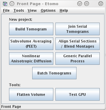
When Etomo is first started, a Front Page panel will come up (shown
above), allowing you to select the operation you want to perform with
Etomo. At this point you can either start working on a new data set by
pressing the Build Tomogram button or open an existing data set under
the File menu or Recent Projects submenu.

However, the first time you start Etomo, you should check for whether parallel processing is set up. This will allow you to distribute some processes across the multiple cores available in your computer. Select Settings under the Options menu. If Enable parallel processing is checked, you are all set. If it is disabled and checked, it means that available computers have been listed in a system-wide file, and the table that you see when you use parallel processing will be different from what is shown here. If the box is not checked, check it and adjust the # of true CPU cores if necessary. Etomo has filled this box with the number of physical cores in the system. Press Done. In this case you can ignore the message about exiting Etomo and proceed.
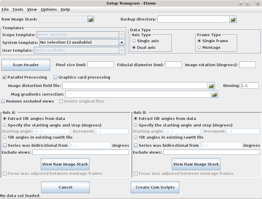
Press Build Tomogram and the Setup Tomogram panel will come up (shown above). A Project Log window will also open that will accumulate the most useful output from the log files at particular steps, as well as error messages and warnings.
To start working on a new data set, the following fields must be filled out. The Raw image stack is the name of the file containing the raw tilt series (or the file from the A axis if a dual axis data set was collected). Enter the Raw image stack by clicking on the yellow file selection button associated with the Raw image stack field and selecting the file. The Backup directory is an optional field to save small working files every time you run a procedure. This field can be left empty if you don't wish to use a backup directory.
In the Templates box, select the plasticSection.adoc System template. This template is part of the IMOD installation and it can be used to set some parameters that are appropriate for this kind of reconstruction.
Select whether the data set is Single axis or Dual axis. The Montage option is available for processing montaged tilt series.
The next fields are Pixel size (nm), the gold Fiducial diameter (nm) and Image rotation (degrees). Pixel size (in nm) is dependent on the microscope, camera, and magnification. The Image rotation (tilt axis angle from vertical, in degrees) will also vary based on the microscope and magnification. Pressing the Scan Header button will retrieve the Pixel size and Image rotation values if these are specified in the file header of the raw stack. For this tutorial example, press Scan Header to define the pixel size for this data set (1.009) and Image rotation (-12.5). You must specify 10 nm for the the gold Fiducial diameter..
The checkboxes for making output be half-size floats are useful for saving storage space when your raw stack is 32-bit floating point, but provide no advantage with this data set, for which the output will be 16-bit integers.
If the Parallel Processing checkbox is enabled, check it so that your screen will look similar to the ones shown here. If calibrations for distortion corrections are available on your system, you will see Image distortion field file and/or Mag gradients corrections entries; leave these blank.
Specify the source of the tilt angles for either one or both axes, as appropriate in the Axis A and, if necessary, the Axis B box(es). In this example, tilt angles are stored in the extended header and so the default Extract tilt angles from data should be used. If you are reconstructing a tilt series that was taken in two directions from zero degrees, you can turn on Series was bidirectional from, and this will take care of setting some appropriate alignment parameters. You can also optionally specify individual projections to exclude from processing steps. The syntax for this exclude list is a comma separated list of ranges (e.g., 1,4-5,60-70). If you do exclude views, you can turn on Remove excluded views in the section above to avoid carrying these views through into various intermediate files, which can be confusing. Notice that there is a also a button in this section to open the raw data file for viewing in 3dmod.
It is useful to look at the raw tilt series files in order to make decisions about preprocessing steps or to see if there are any particular views that have poor image quality, and that you want to exclude from the alignment and reconstruction.
To determine if you have views that have poor image quality (poor focus, etc.), open the raw stack(s) by pressing the View Raw Image Stack button(s). Movie through the raw tilt series images by clicking the middle mouse button. Notice how the images jump around slightly. Make note of any particular views that you want to exclude from the alignment and reconstruction. In this sample data set, there are no images that need to be excluded.
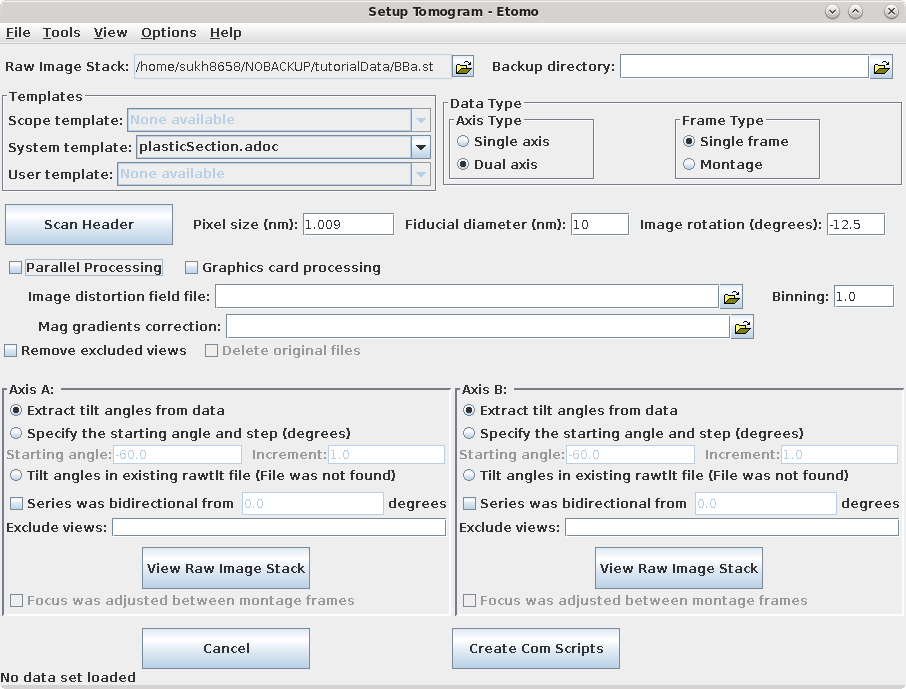
Details specific for the tutorial sample data set are shown above. For this sample data set, the Raw image stack is BBa.st; it is a dual axis set. The pixel size is 1.009 nm, the Fiducial diameter is 10 nm and the image rotation is -12.5 degrees. Tilt angles for this data set are stored and extracted from the image file.
Press the Create Com Scripts button to move on to generating the tomograms.
If you need to exit Etomo before finishing this tutorial, you can continue
where you left off by going to the tutorialData
directory, which now contains your data set, and typing:
etomo BB.edf
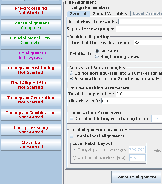
The Main Window consists of several areas: on the left is a column of buttons
(Process Control Buttons) that allow you to select a particular stage of
tomogram computation to work on. On the top is a Process Monitor that informs
you of the status of the current process or the last process completed. To the
left of the Process Monitor are the Axis Buttons which allow you to move
between Axis A and Axis B. The Main Window is currently open to Axis A.
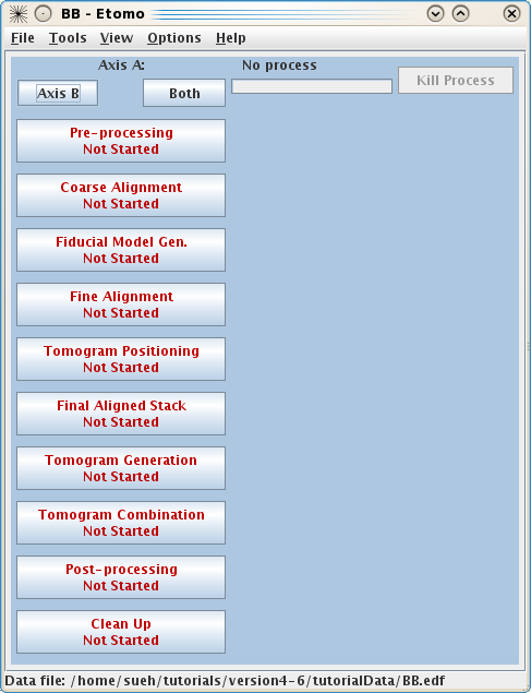
The Process Control Buttons are arranged in the suggested order of processing from top to bottom. The buttons are color coded to signify the stage of the process, where red indicates that the process has not been started, magenta indicates that the process is currently in progress, and green indicates that the process has been completed. When one of the buttons is selected, the right side of the window will fill in with information and fields associated with a specific process. These forms are referred to as Process Panels. They allow you to modify the necessary parameters and execute specific programs required by that processing step. The parameters and buttons on each Process Panel are typically laid out from top to bottom in the order they should be executed, much like a flow chart. When you execute a process (by pressing a button on one of the Process Panels) the Process Monitor will indicate what the process is doing and when it is complete.
If images were collected on the microscope using a CCD camera, random x-rays hitting the CCD camera during collection of the initial dark reference or individual images can cause extreme high or low pixel values in your data file. As a result, these extreme values ruin the contrast and can cause artifacts in the reconstruction. CMOS cameras have similar effects, although not as extreme if the camera is read out many times for each exposure; they also have a tendency to have "hot" pixels that produce extreme values. The example in this tutorial does not have very extreme pixel values that would cause serious problems; in fact no pre-processing is needed for the first axis. We will thus skip over to the second axis to illustrate the procedure for assessing the extent of extreme values and removing them if necessary.
To see the B Axis, press the Axis B button at the top of the Etomo window. This will bring up another set of process buttons on the left, which can be used to perform the operations for aligning the Axis B tilt series and calculating the tomogram. To prevent confusion, Axis A has a blue background and Axis B has a green background.
Next press the Pre-processing button to open the panel for removing artifacts.
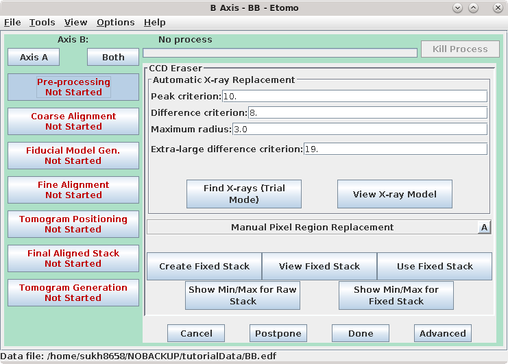
Press the Show Min/Max for Raw Stack button to run clip stats, a program which displays the minimum and maximum densities for each section of the raw stack. Windows will open with the text output and with a graph of these densities.
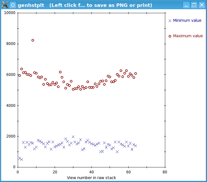
If the minimum density value is a negative number or 0, then you probably have an extreme black pixel in your data set, caused by an x-ray event during collection of the dark reference. If some sections have a high maximum density, then you have extreme white pixels in your data set. In this case, there is one obvious outlier and some other maxima that stand out above other nearby values, although the latter differences are small.
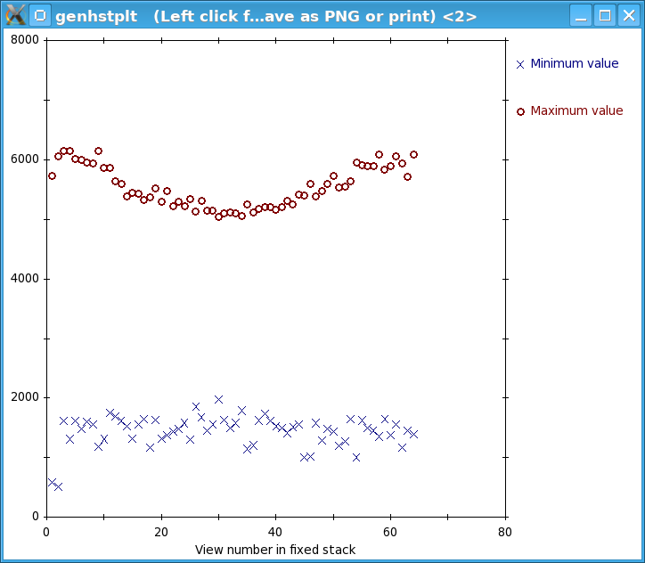
Press the Create Fixed Stack button to create a second stack with X-rays removed.
Press the View Fixed Stack button to view that stack, and press the Show Min/Max for Fixed Stack button to run clips stats on the fixed stack. In the graph, notice that the big outlier has been removed and that the maxima are generally more consistent from one view to the next.
In general, if the contrast appears good in the display without the Black and White sliders in 3dmod being very close together, and the outliers from the raw stack clip stats output are gone from the fixed stack output, then the removal is adequate. Since that is the case here, press the Use Fixed Stack button. Close the statistics and graph windows and press the Axis A button to return to the first axis.
The procedure when the removal is not good enough is to reduce both the Peak criterion and the Difference criterion by one, and create a new fixed stack. For details on this operation, refer to the PRE-PROCESSING: REMOVING X-RAYS section of the Tomography Guide.
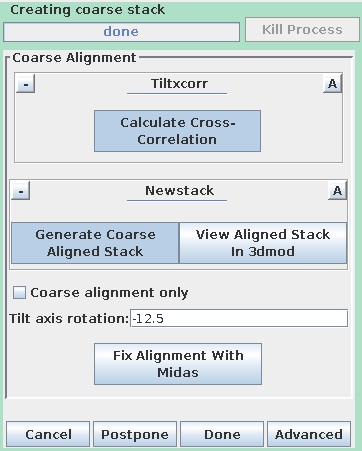
Press the Coarse Alignment Process Control Button to proceed with creating a coarse-aligned stack.
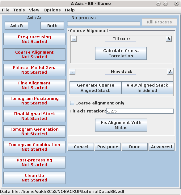
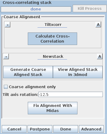
Pressing the Calculate Cross-Correlation button runs the program,
Tiltxcorr. The program uses cross-correlation to find an initial translational
alignment between successive images of a tilt series (i.e. just shifts in x and
y). The output file, BBa.prexf, contains a list of transforms (or recommended
shifts) that will be applied to the image data in the next step.
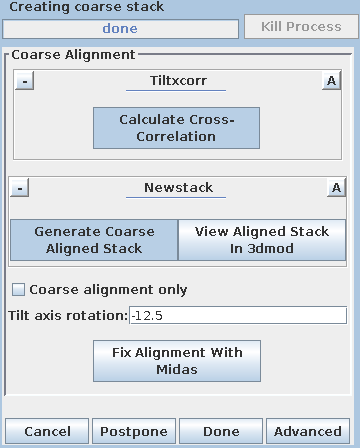
Pressing the Generate Coarse Aligned Stack button will run 2 programs. Xftoxg takes the transforms created by Tiltxcorr to obtain a single consistent, or 'global' set of alignments. These new transforms are then applied to the image data using the program Newstack. The output file created is BBa.preali. One can view the prealigned stack by pressing the View Aligned Stack in 3dmod button. Large image shifts can be edited manually using the interactive program, Midas. This is not an issue with this data set; see the COARSE ALIGNMENT section of the Tomography Guide for details. The Tilt axis rotation entry is used if Midas is run, because Midas will rotate images so that the tilt axis is vertical. The Binning in Midas entry is useful with images of ~4K pixels or larger, because initially binned images will look better im Midas than ones zoomed down for display. The Coarse alignment only check box can be selected for making a tomogram without a fiducial alignment; see Making a Quick Tomogram with Correlation Alignment in the Tomography Guide for details. Once you are satisfied with the prealigned stack, press the Done button to proceed to the next step.
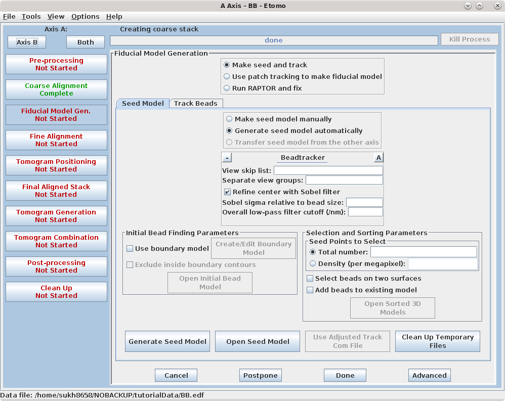
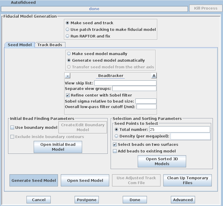
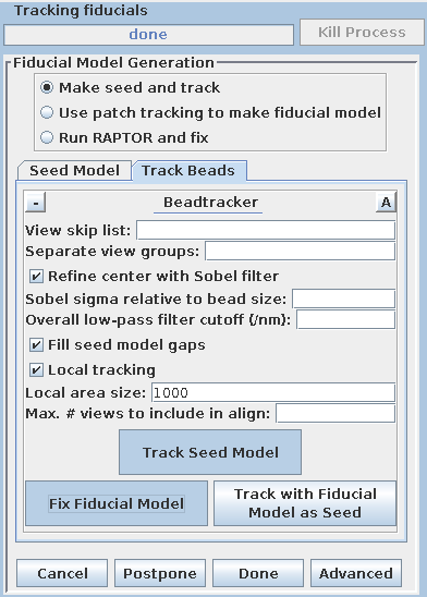
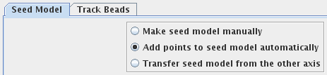
There are three options available to generate a fiducial model. The most common is to Make seed and track a number of gold fiducial markers, where the starting points can be selected either manually or automatically. These starting points are referred to as a seed model because they are picked on only one section, and the fiducials are tracked from there. The option, Use patch tracking to make fiducial model, can be used if the data set does not contain gold fiducial markers or too few gold fiducials. Run RAPTOR and fix will use a program developed at Stanford to automatically find and track gold fiducial markers through the tilt series. See the FIDUCIAL MODEL GENERATION section of the Tomography Guide for details. We are first going to select seed points automatically, using a newer feature. Then we will back up and go through the older method, which is better for illustrating the procedures you would need to follow with more problematic data sets.
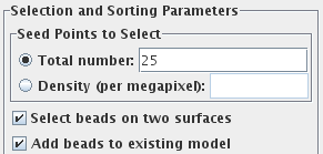
Enter 25 for the Total number to track, and turn on Select beads on two surfaces.
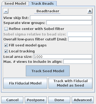
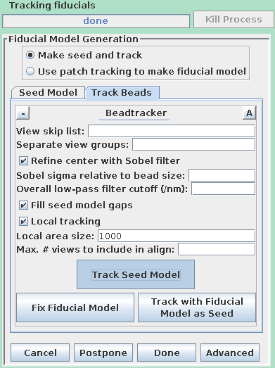
Select the Track Beads tab.
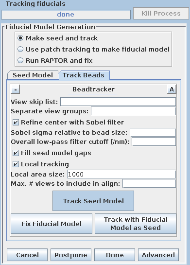
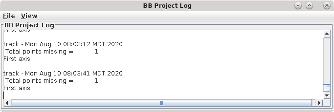
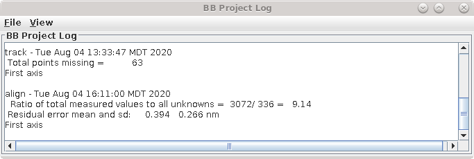
This will run the Beadtrack program to find the gold on all other sections. The output file created by tracka.com is BBa.fid, which is the completed fiducial model. This computer-generated model is not perfect, and gaps in the fiducial model can occur. A report of the total points missing will be indicated in the Project log window. If a large number of points are missing, press the Track with Fiducial Model as Seed button, which will rerun the tracking program with the fiducial model as the seed. For this sample data set, no more points will be filled in.
If points are still missing, the next procedure involves an iterative process to edit this fiducial model. Note, that it is not necessary to fill all the gaps, particularly if there is a good excess of fiducial points, as there is here. However, it is important to make sure that the large majority of the fiducials are tracked all the way to the two ends of the tilt series.
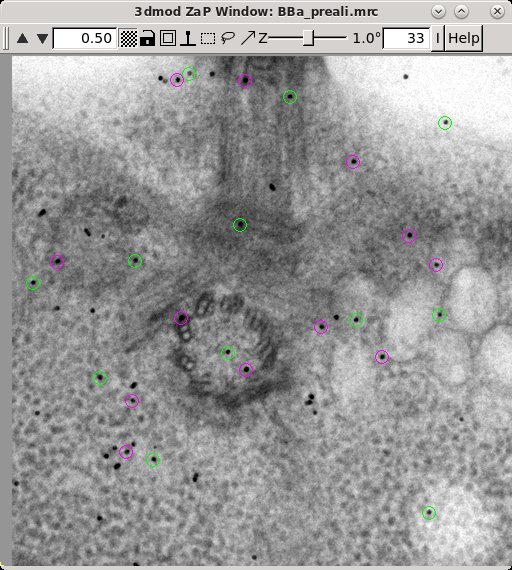
This procedure will open the prealigned stack (BBa.preali) and the fiducial
model file (BBa.fid) in 3dmod. (Note: for the rest of this tutorial, we will
show large images at a zoom of 0.5 instead of 1 to save space, but they will
show up at zoom 1 for you unless you have a high-resolution monitor.)
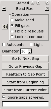
The Bead Fixer dialog box will come up in Fill gaps mode. The Bead Fixer facilitates editing the fiducial model.
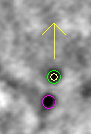
Click the Go to Next Gap button (or use the spacebar as a hot key). This will attach to a point (highlighted with a yellow circle) that has a missing model point on an adjacent section. Use the Page Up key (when an up arrow appears above the point) or the Page Down key (when a down arrow appears above the point) to find the section with the missing point and use the second mouse button to add the point in the center of the gold particle. It is useful to increase the magnification of the image with the '+' key and adjust the contrast on the sections, especially at high tilt.
Repeat 'Go to Next Gap' until the message, 'No more gaps found' comes up in the main 3dmod window. Save the model file by going to File -> Save model, or by hitting the hot key 's', and press the Done button to advance to the fine alignment step.
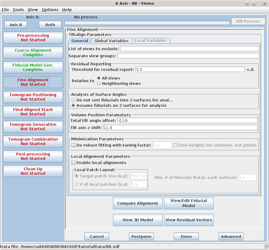
The Fine Alignment panel is organized with a set of three tabs to solve for various alignment parameters. A general alignment is first done by pressing the Compute alignment button at the bottom of the Fine Alignment box.
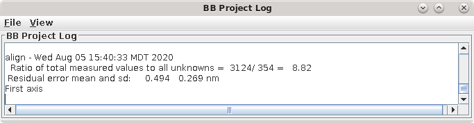
This command file runs the program, Tiltalign, to solve for the displacements, rotations, tilts and magnification differences in the tilted views. The program uses the position of the gold particles in the fiducial model and a variable metric minimization approach to find the best fit. It creates a log file that gives a synopsis of what was done. A report of the Ratio of total values to all unknowns, the Residual error mean and sd, and the Global leave-out error is displayed in the Project Log window. To access the full log file, right click the mouse cursor over the window region associated with the process. This will open a menu that is split into three or four sections: the first section will allow you to open the log files associated with the current process; a second section allows you to see graphs of alignment parameters, but is not present on most other panels; the next section will allow you to open up the man pages associated with the current processes, and the final menu section opens the general help guides. Select "Align axis:a log file" to open the log file. This will open a tabbed file that contains the complete log and short sections from this log file. In my example, the first Compute Alignment run gave a Residual error mean of 0.394 nm and a global "leave-out" error of 0.4491 nm.
Both of these error measures need some explanation. The residual error is
the kind of error that you may be familiar with from other situations where data
are fit to equations. After the best-fitting solution is found, the
distance between the fiducial position implied by the equations and the actual
position is computed for each point included in the fit. The mean residual
error is the mean of these distances. A "leave-out" error, on the other
hand, indicates how well the solution would predict the location of points
not included in the fit. It is computed by repeatly leaving some
points of out the fit and measuring how well the solution fit to the rest of the
points predicts the points left out. As you can see from the output, many
thousands of points have to be left out get a good estimate of leave-out error.
This process is referred to as cross-validation. It is important to pay
attention to leave-out error because you want a solution that aligns your
specimen well in general, not just at the points being fit. Fitting to
equations with more variables will virtually always reduce the mean residual,
but at some point the equations will be fit excessively to the noise in the
measurements and give poorer predictions of other positions. This is
called overfitting, and the leave-out error will rise when this occurs.
Whenever you change alignment options, you should use the leave-out error to
decide if the change was a good one or produced overfitting. When
adjusting fiducial positions, as in the procedure to be done next, you can still
use the mean residual as a guide for how well the changes improve the solution.
This result is too good for illustrating further steps, so now we are going to back up. First exit from 3dmod, and then go to the terminal window and remove or rename the seed mode, for example:
mv
        BBa.seed BBa_auto.seed
Next, in Etomo, press the Fiducial Model Gen. button on the left, select the Seed Model tab, and switch back to Make seed model manually so that the screen looks like this:
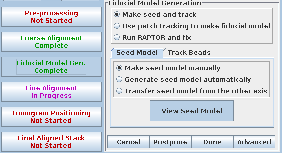
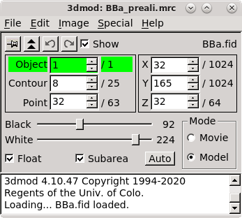
(This button was originally labeled 'Seed Fiducial Model' before any model was created.) This will open BBa.preali in 3dmod and create an empty model file named BBa.seed. It will also bring up the Bead Fixer dialog box in Make seed mode with Autocenter checked. Check Automatic new contour if it is off; 3dmod will remember this setting from session to session.
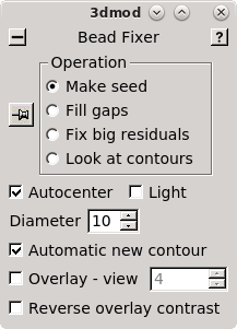
3dmod will open the file to the middle section (section 33 in this tutorial stack). You can return to the middle section by pressing the Insert key on your keyboard (use Shift-Home on Mac).
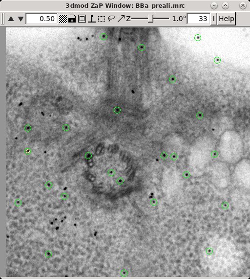
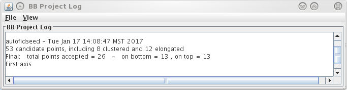
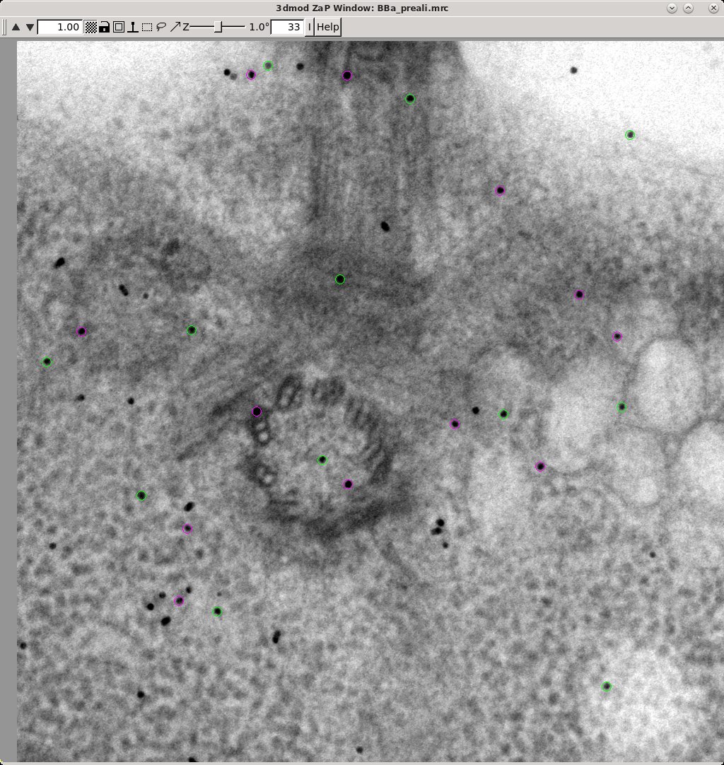
In the Zap (image) window, place a model point in the center of 20-30 gold particles by centering the cursor in the middle of the gold particle and pressing the second mouse button (this is the middle mouse button by default, but you may have remapped the mouse buttons in 3dmod). Because Automatic new contour is checked, a new contour for each new gold bead will be created. Because Autocenter is checked, 3dmod should make sure that the model point is positioned in the center of the gold bead, so you do not need to be as careful as when filling gaps. In my example (BBa.seed) I selected 25 gold particles; the model contains 1 object, 25 contours, with each contour having 1 point. Save this seed model.
Next, select the Track Beads tab again. In order to keep the result from being so good this time, turn off Refine center with Sobel filter.
Press Compute Alignment. This time the
residual and leave-out errors are quite a bit bigger.

The goal of the fine alignment step is to reduce the residual error mean to
0.2 - 0.5 nm for the pixel size of this tutorial data set. When expressed in
nanometers like this, the residual error means that can be achieved will
tend to scale with the pixel size, but not proportionally, especially when going
to smaller pixel sizes where various limitations will keep the error from going
below a certain level.
The Tiltalign program also creates two model files that provide useful information about the fiducial model. The first (BBa.3dmod) displays a 3-D model of the fiducials based on their solved positions. Fiducials that are present on the two surfaces are assigned 2 different colors; pink spheres on one side and green spheres on the other. Examine this model by pressing the View 3D Model button on the bottom of the Fine Alignment box:
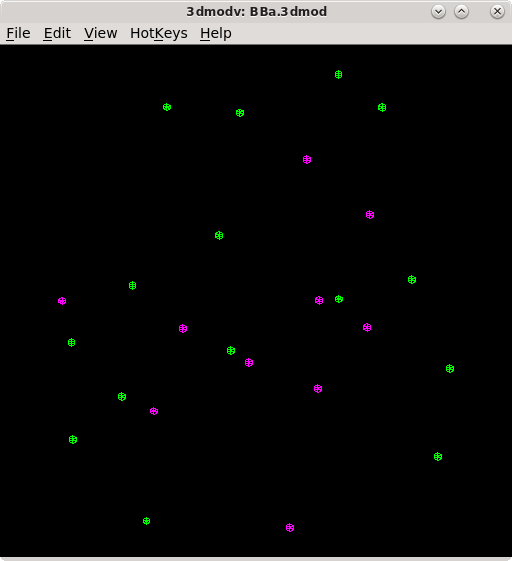
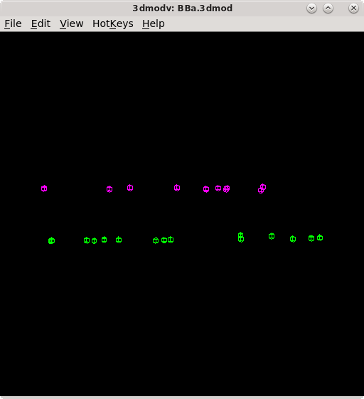
You should see a nice distribution of pink and green spheres across the field of view. Rotate the model to view edge-on by holding down the number 8 key on the keypad. You will see the separation of the two surfaces with this view. Avoid using models that have a cluster of fiducials in any one particular region because this will skew the alignment. Close the 3dmodv window.
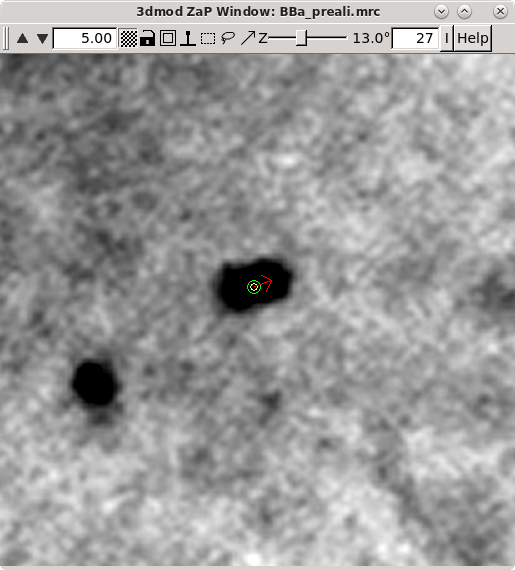
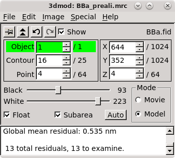
The second model Tiltalign produces is a residual vector model. Press the 'View Residual Vectors' button at the bottom of the Fine Alignment box. This will open the prealigned stack in 3dmod and display the residual vector model on each section.
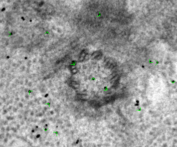
The model will show the current model point as the origin of a green arrow, and
the position of the residual as the end of the arrow. This residual
displacement is expanded by a factor of 10 in order to distinguish it from the
actual model point, because displacements are often very small (< 2
pixels). In large (>2k x 2k) images the residual model will often show large
displacements in one area but not in other areas. In these cases, the residual
model helps to make decisions if local alignments are needed. In this example,
local alignments are not needed. It is common to have larger residuals at the
higher extreme tilts. Leave 3dmod open for the next several steps and press the
'View/Edit Fiducial Model' button to reload the fiducial model for
editing. This will bring up the Bead Fixer dialog box in Fix big residuals
mode and load the aligna.log file.
Note that you may be able to get essentially as good a result by using "robust fitting" instead of fixing fiducial points. Robust fitting will give less or no weight to a small fraction of points with high residuals so that they do not influence the alignment solution, so if the remaining points are numerous enough to give a good solution, the alignment should be adequate. See the see the Using Robust Fitting section of the Tomography Guide for details.
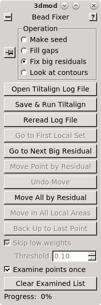
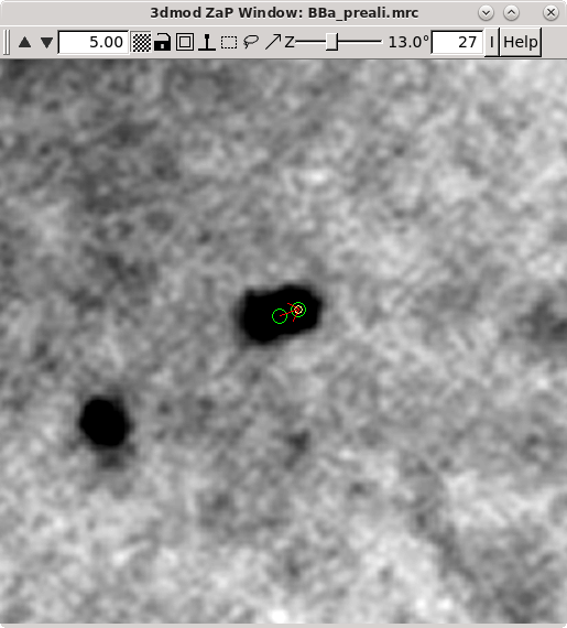
Click 'Go to Next Big Residual' in the Bead Fixer dialog box.
The model point that had the big residual will have a red arrow pointing in the direction of the recommended move. You'll probably be able to see that the model point is not centered properly on the gold. If you click 'Move Point by Residual' in the Bead Fixer dialog box, it will move the model point by the recommended amount. This works most of the time, but if the recommendation looks wrong, you can move it by hand by centering the cursor over the middle of the gold bead and then clicking the third mouse button. The recommendation is the position predicted by a mathematical alignment model fit to all of the fiducial model points and is not based on an analysis of where the bead is actually located in the image. If you have a specimen that is distorted enough so it does not fit the alignment model well, then arrows will often point away from the actual gold positions.
Repeat selecting 'Go to Next Big Residual' and 'Move Point by Residual' until no residuals are found. The hot key ' will cycle to the next residual and the hot key ; will move point by residual. The goal is to center each point over the fiducial it is associated with. The residual arrow is not always correct. Points can also be moved with a right mouse button click. Sometimes a fiducial from the other surface will make it difficult to see the extent of the current fiducial. Use the Page Up and Page Down buttons to distinguish fiducials (but always return to the section selected by the Go to Next Big Residual). You can undo moving by the residual by pressing the Undo Move button.
When there are no more residuals to fix, save the model file and leave the file open.
Access the aligna.log file and go to the Surface Angles tab.
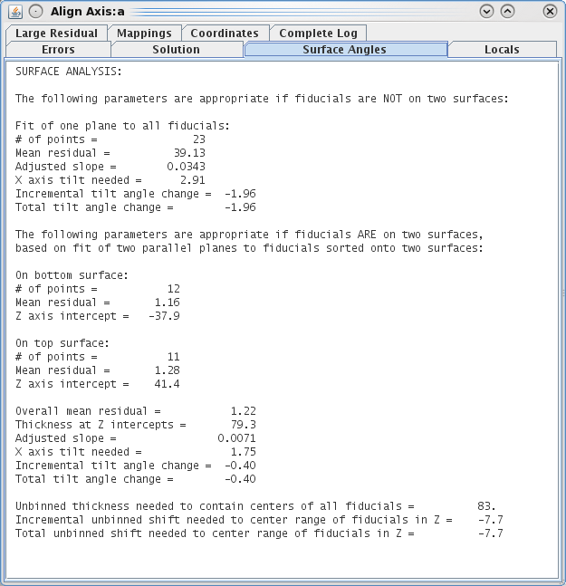
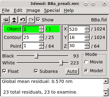
Note the "Total tilt angle change" near the bottom (in my example, this value was -0.45). Put this value in the Fine Alignment Volume Position Parameters box under Total tilt angle offset. Press the Compute Alignment button again. The alignment will be computed with your corrections incorporated, and 3dmod will reread the resulting log file. See the text box at the bottom of the main 3dmod window.
Proceed again to fix model points with large residuals. Save the model.
If your data set has a good distribution of gold on both surfaces, you can solve for distortion. Press the 'Global Variables' tab in the Fine Alignment box:
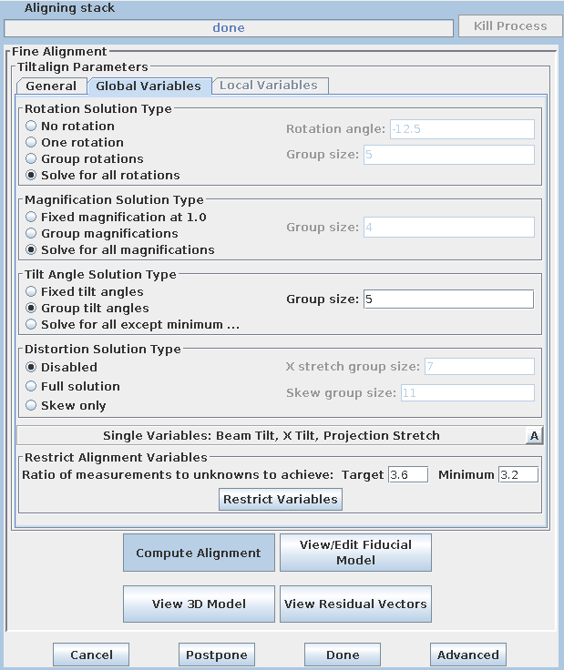
Select the 'Full solution' option in the Distortion Solution Type area at the bottom of the panel. This will activate solving for two variables that together represent a shrinkage or stretch along an arbitrary axis: X-axis stretch and Skew. Keep the default group size and hit the 'Compute Alignment' button to run the alignment. 3dmod will re-read the log file when Compute Alignment is done. Notice that both the mean residual and the leave-out error dropped, this indicating the value of this change.
Return to the 3dmod windows and repeat fixing the new residuals that Tiltalign came up with after solving for distortion. Then press the Save & Run Tiltalign button in the Bead Fixer window to save the model and compute the alignment. You can use this button to avoid having to go back to Etomo, as long as you haven't changed any parameters in Etomo. After a few runs of running the alignment and checking model points in 3dmod, the final mean residual should come down to 0.2-0.4. In my example, the final Residual error mean was 0.562 nm because I did not do much refinement on this revision.
Now that you have finished fixing fiducial positions, there is an important but simple step to prevent overfitting. Select the General tab and press Run Cross-Validation in the Restrict Align Variables with Cross-Validation box. This runs the program Restrictalign, which will test different combinations of alignment options to optimize the leave-out error by increasing the amount of grouping or leaving a variable out completely. Eventually, the result is reported in the project log. In my case, .601 nm. Etomo reads in the changed alignment command file and updates the options in the interface.
The goal of the next step is to shift and rotate your reconstruction so that
it is as flat as possible and will fit into the smallest volume. This is done
by sampling three regions of the tomogram, ones computed from near the top,
middle, and bottom of the tilt images. (When these samples are not adequate,
you can do this instead with a whole, binned down tomogram; see
Positioning with a Whole Tomogram in the Tomography Guide for
details.) There are two rotations which can be adjusted: the rotation
about the tilt axis, to make the section level when viewed in the X-Z plane;
and a rotation about the X axis, to make the section come out at the same Z
height throughout the length of the tomogram.
There is a feature that allows the top and bottom surfaces of the section to be detected automatically, which saves drawing a model to define the surfaces. We will go through doing this operation manually for this axis; we will use the automatic positioning feature for the second axis.
Set the Positioning tomogram thickness to 400. This will create a reconstruction that is much thicker than the original section.
Press Create Sample Tomograms
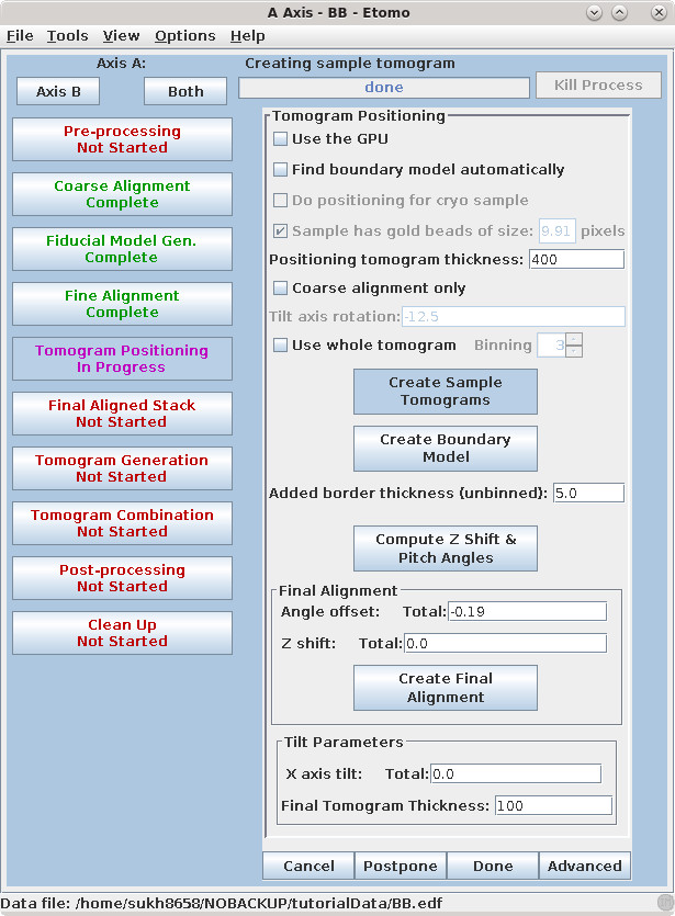
This command file first extracts and aligns a 60 pixel sliver from the top, middle, and bottom of the image stack. The program then uses these samples to create 20 slices of the reconstruction from the top, middle, and bottom of the aligned stack. These output files are named topa.rec, mida.rec, bota.rec. Press Create Boundary Models.
When the 'Create Boundary Models' is pressed, 3dmod will read in all three reconstructions at once, with the topa.rec displayed first and viewed edge on. 3dmod will also start with an empty model, named tomopitcha.mod.
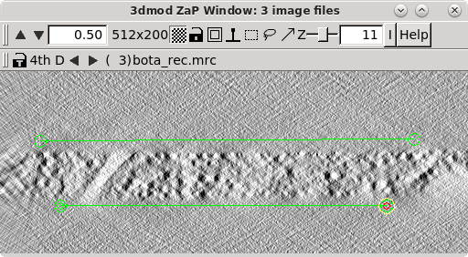
The top bar of the Zap window has a feature '4th D' and a backward and forward arrow. If you click the forward arrow, you can cycle through to the mida.rec and bota.rec reconstructions, respectively. Start with the topa.rec. Use the contrast sliders to adjust contrast. Notice the material in the center of the volume with a mottled appearance. This is the part of the reconstruction with biological material. Using the middle mouse button, place one model point at the left side of the top surface that defines the region containing the biological material, and a second model point at the right side of the top surface. A line will connect the two points. Model the bottom surface of the section with 2 points on the left and right sides, respectively. Toggle to the mid.rec and bot.rec file by hitting the arrow button to the right of '4th D' at the top of the zap window. Repeat modeling the top and bottom surfaces of the other two reconstructions. The final model should have 1 object and 6 contours, and each contour should have 2 model points. Save this model file.
It is generally helpful for the thickness of the final tomogram to be about 10 to 20 pixels greater than the actual distance between the lines that you draw. You can adjust the entry in Added border thickness to accomplish this. The default value of 5 will make the tomogram 10 pixels thicker; change it to 10 to make it 20 pixels thicker.
Based on these model contours, tomopitch determines parameters to make the
reconstruction as flat as possible and to fit in the smallest volume as
possible. These offsets are automatically added to the existing Angle
offset, Z shift and X axis tilt values. The Final tomogram
thickness is also entered by Etomo from the tomopitch log.
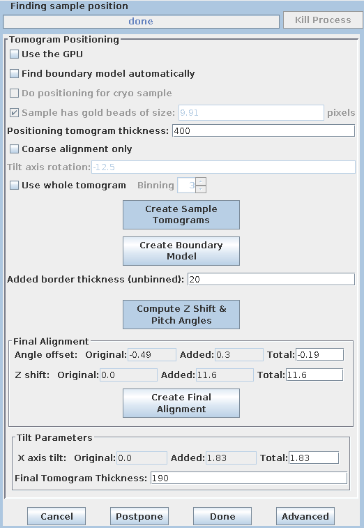
Press the Create Final Alignment button. After the final alignment transforms are created, press the Done button to advance to the next step.
Press Create Full Aligned Stack.
This command will apply the alignment transforms to the full-sized image for the final, aligned stack. The output file is named BBa.ali
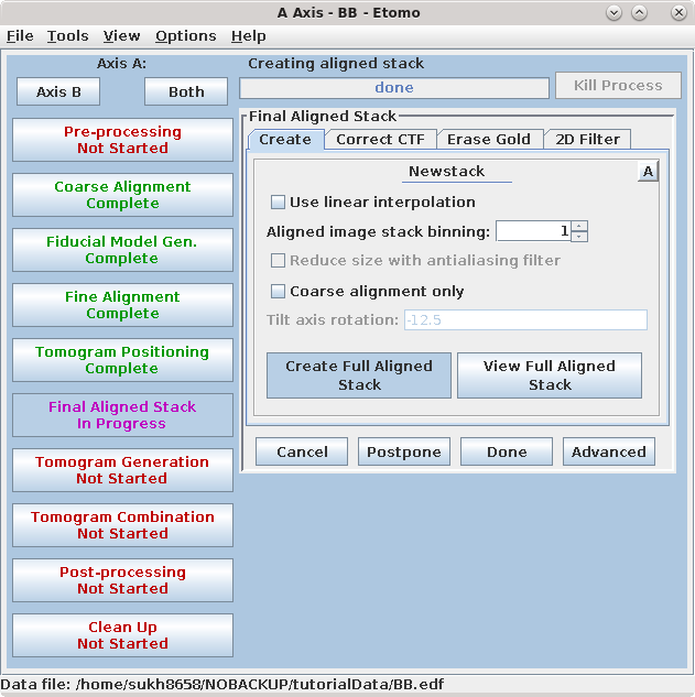
The full aligned stack may be viewed by pressing View Full Aligned Stack, although this is not necessary. There are optional steps for CTF correction, erasing fiducials, and filtering the aligned stack, which are also not needed here. Press the Done button to advance to the next step.
The default filtering parameters in the Tilt Parameters section are appropriate for many cases, but can be changed, or the aligned stack can be filtered, to reduce noise in the reconstruction (see the TOMOGRAM GENERATION section of the Tomography Guide for details).
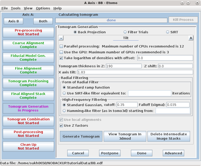
Select some number of cores in the Parallel Processing table.
Press Generate Tomogram. First, Etomo runs a program called Splittilt, which divides the computation into a multiple command files, called chunks. Then it starts running the chunks, and the progress bar will report how many have completed.
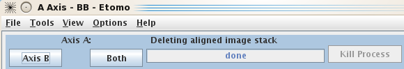
When the tomogram is computed, examine it by pressing View Tomogram in 3dmod. You may also choose to Delete Intermediate Image Stacks at this point to save space.
Movie through the reconstruction by hitting the second mouse button to step through serial, tomographic slices from the top surface of the tomogram to the bottom surface.
To see the B Axis, press the Axis B button at the top of the Etomo
window. Since we already did the Pre-processing step for this axis, go to the Coarse Alignment steps, as described
above for Axis A.
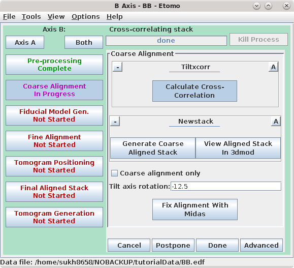
After the coarse-aligned stack has been generated, press Done to
advance to the next step.
In order to combine both tilt axes at least some (8-10) of the beads that you
track must be the same in the two series. To accomplish this, use the program
Transferfid.
Pressing the Transfer Fiducials From Other Axis button will run a program, Transferfid, that creates a seed model for the second axis based on the fiducial model from the first axis. The program will search for the pair of views in the two series that correspond the best, then transfer the fiducials from the first series to make the seed model for the second series. At the end, the program will list the fiducial correspondence between the first and second axes and will report this in the Project log window.
Do not worry if a few fiducials failed to transfer. In this example, 17 fiducials correspond:
Press Add Points to Seed Model to add some more points to the seed model produced by Transferfid, which is named BBb.seed. Select the Track Beads tab and proceed to Track Seed Model in the Axis B window.
This will automatically track the fiducials for the 'B' set. Fix the gaps in the BBb.fid file by pressing the Fix Fiducial Model Using Bead Fixer as outlined above for the A axis. When the gaps are fixed, press Done to proceed to the Fine Alignment and Tomogram calculation steps.
You will now proceed with the same steps following the same procedure as outlined above for the Axis A set. Briefly:
At this point, you will start the iterative alignment procedure as you did for the 'A' set by editing model points with large residuals, saving the model, and computing the alignment. Use Run Cross-Validation to optimize the alignment variables. When the alignment is complete, press Done and proceed with the tomogram generation steps.
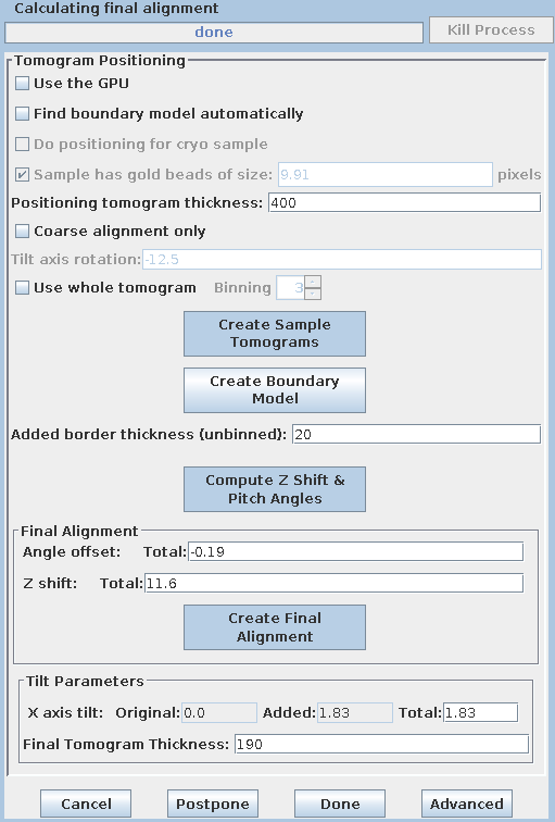
To use the automatic positioning, turn on Find boundary model automatically and set the Positioning tomogram thickness to 400 again.
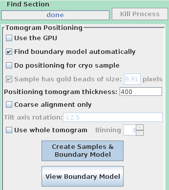
Notice that the buttons have been relabeled to Create Samples & Boundary Model and View Boundary Model. The automatic tomogram positioning can be done with either samples or a whole tomogram, and the whole tomogram is more reliable when there is not enough material in the standard sample locations. We will still use samples here because somewhat different methods are needed to examine the boundary model from a whole tomogram (see the section on automatic positioning with a whole tomogram in the Tomography Guide for details.)
Press Create Samples & Boundary Model. Press View Boundary Model when it is done and examine the contours that it drew.
Proceed with 'Final Aligned Stack' steps as outlined above for the A Axis.
Proceed with 'Tomogram Generation' steps as outlined above for the A Axis.

Go back to the A Axis by pressing the Axis A button.
To combine the two tomograms press the Tomogram Combination process button.
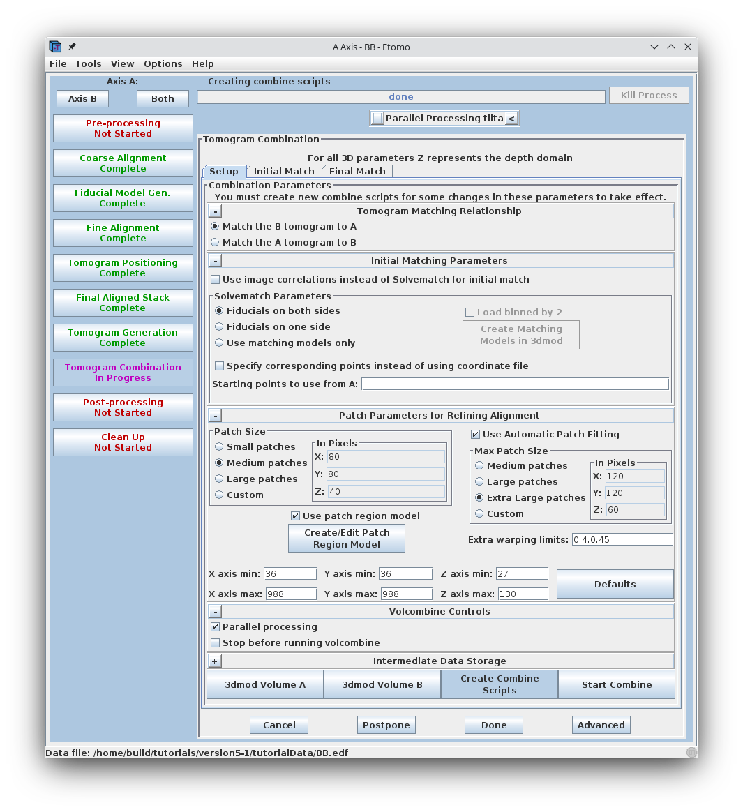
The Tomogram Combination Panel is organized with 3 tabs: Setup, Initial Match, and Final Match.
The Setup window is where information is given about the particular data set. The first section describes the Tomogram Matching Relationship. It is most common to match the B tomogram to A.
The Solvematch Parameters box asks for information on the fiducial marker distribution. In this example, fiducials are on both sides. For this data set, the programs will have no trouble fitting to all of the points at once, so it is not necessary to fill out Starting points to use from A.
The next section contains information for Patch Parameters for Refining the Alignment using local 3D cross-correlations. Select Small patches. Either Medium patches or Large patches are needed for most data sets, but this data set has been binned to reduce its size, so small patches have plenty of information in them. Note that Use Automatic Patch Fitting is checked. This feature automatically increase the size of the patches if not enough information is found. Patch size won't be increased unnecessarily.
When automatic patch fitting is selected, the programs also analyze the amount of information present thoughout the volume and try to exclude patches that do not have enough information. If this procedure does not work well enough, then you would have to fall back to the older methods of indicating the areas from which to extract patches. To give you some experience with these methods, we will go through the procedure for setting coordinate limits for the volume.
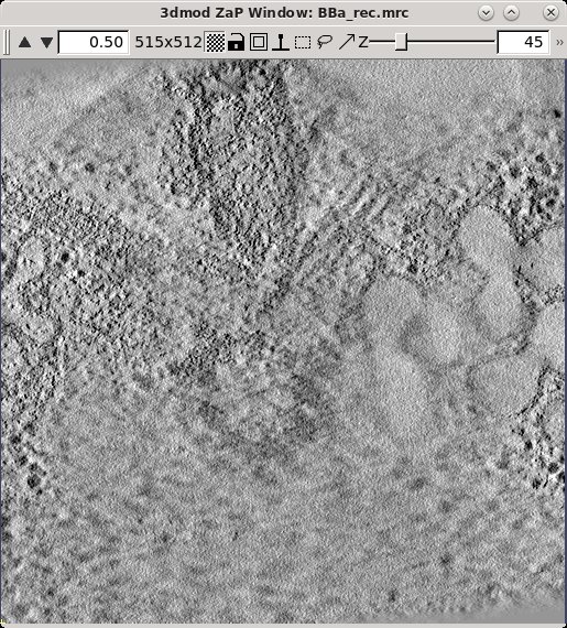
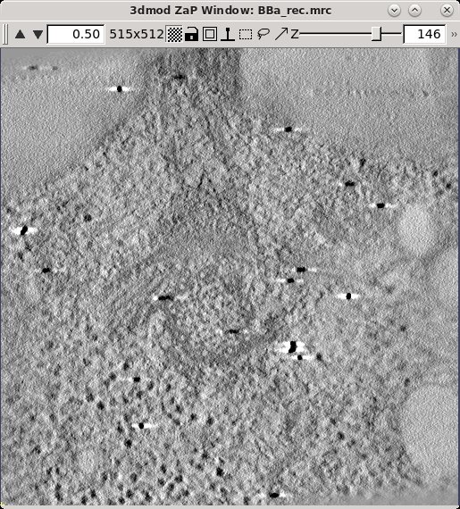
When it is necessary to specify the limits of the volume from which the patches will be extracted, it is important to look at the tomogram being matched to. Using the entire Z axis range will almost never work without automatic patch fitting, and even for the X and Y axes it may not be good to use the defaults. To find the limits, press the 3dmod Volume A button at the bottom of the panel. This will open BBa.rec in 3dmod. Step through the images and decide what range of the X axis, Y axis and Z axis contains useful information for matching up the volumes. In this example, defaults were kept for the X and Y axis.
In this example Z axis min and Z axis max were set to the first and last slices where about half the material in the slice is not blurry (27 and 130).
Sometimes, just setting coordinate limits will not eliminate "empty" regions well enough to allow the two axes to combine. In that case, you have to make a patch region model. To make a patch region model, check the box Use patch region model and press the Create/Edit Patch Region Model button to open up the axis that is being matched to. In model mode, trace closed contours around the areas that contain biological material. Do this every 10 slices or so in the tomogram. Save the model, which is named patch_region.mod. Creating the patch region model is particularly useful when reconstructing data sets that have large amounts of resin or open areas in the images. This example data set does not need a patch region model.
When the parameters for the Setup panel have been entered, press Create Combine Scripts to create a series of command files that will run various programs in the combine procedure. Ignore the warning message that pops up. Press Start Combine to begin the process of dual-axis tomogram combination. Etomo will automatically advance to the Initial Match and finally the Final Match tabs as various programs are being run.
After tomogram combination is complete, press Open Combined Volume to view the final tomogram. Press Done to advance to the final steps.
Post-processing involves a volume trimming and byte scaling step, followed by deletion of intermediate files. There are also options to flatten the volume and to create a reduced and/or filtered volume; both of these can be useful when working with very large data sets, and the flattening is particularly helpful when reconstructing serial sections. A description of their use can be found in the POST-PROCESSING section of the Tomography Guide.
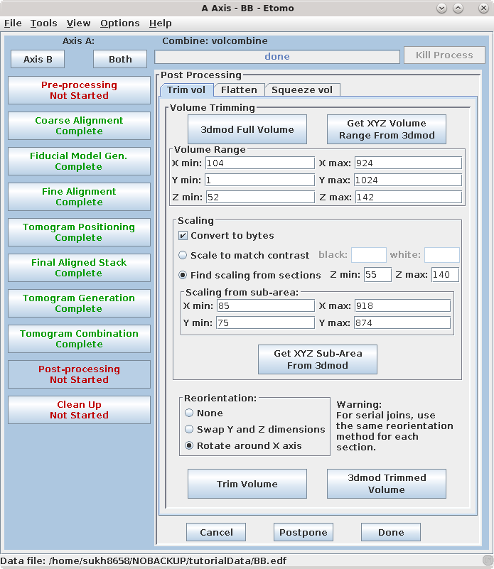
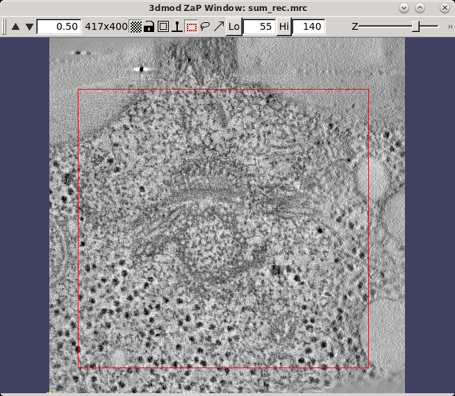
The final reconstruction of the two axes combined into one will always be called sum_rec.mrc. (If you have a single axis data set, the name of the reconstruction file at this point will be the data set name followed by _full_rec.mrc) Open the sum_rec.mrc reconstruction by pressing 3dmod Full Volume. Step through the reconstruction and determine the X,Y and Z ranges for the final volume. A convenient way to set the X and Y range is to turn on the rubberband with the dashed rectangle in the toolbar of the Zap window, press the first mouse button over the upper left corner of the desired area, and drag the mouse to the lower right corner. Z can also be set, if desired; press Lo to set the minimum Z and Hi to set the maximum Z. When you press Get XYZ Volume Range from 3dmod, Etomo will retrieve the X and Y values of the rubberband (and Z values if they are set) from 3dmod. In this example, there is some trimming in X and the default range for Y is used. The Z axis (in the flipped tomogram) range has been set from a Z min of 52 to a Z max of 142 to exclude non-cellular material. Finally a scaling range is set to find the range of slices that exclude the gold beads. In this example, the scaling is section based and has a range between slices 55 and 140 (see below to enter these numbers using 3dmod).
Sometimes it is not possible to find a range of slices that contain no gold. For example, the sample used here contains some gold particles on the plastic resin outside the cell that show up in the same slices that we would like to use for scaling. Limiting the X and Y scaling range to exclude any such gold particles will improve the contrast of the final tomogram. Press the 3dmod Full Volume button and bring up the ZaP Window. Go to a slice which shows gold particles and put a rubberband around an area that excludes them. To do this, press the rubberband toggle to the left of the Z slider.
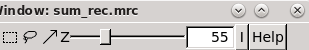
Press the left mouse button over the upper left corner of the desired area, and drag the mouse to the lower right corner. Then move the Z slider to lower part of the scaling range (55) and press Lo. Move the Z slider to the upper part of the scaling range (140) and press Hi.
Go to the Scaling box in Etomo and press the Get XYZ Sub-Area From 3dmod button. This will cause the Etomo to retrieve the X, Y, and Z values you selected. The default reorientation option will rotate the final volume around the X axis so that it can be read in easily by 3dmod and other programs without special options. Press the Trim Volume button to run Trimvol. Trimvol is a single tool for trimming a volume and converting it to bytes. Finally, view the final, trimmed volume (named BB_rec.mrc) by pressing 3dmod Trimmed Volume. Press Done to proceed to file cleanup.
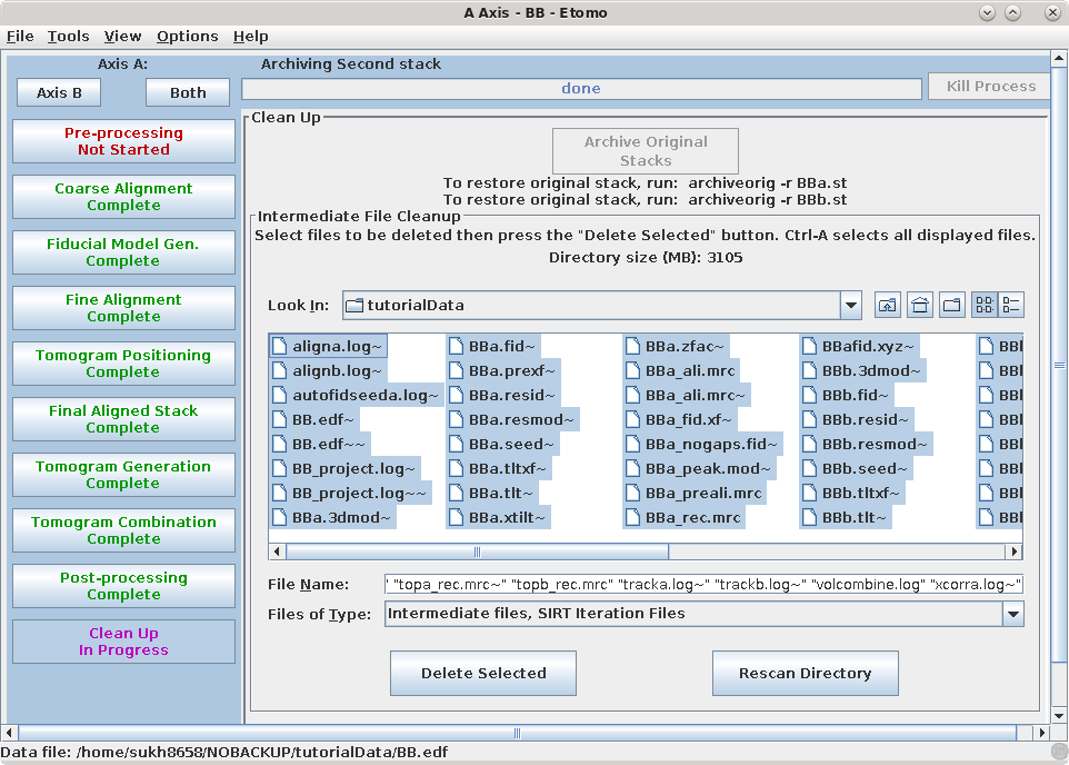
Cleaning up of your files is very important! Since you removed x-rays from one of the stacks, the first step available to you is to "archive" the original stack. This process replaces the original stack by a small, highly compressed file of the differences from the current raw stack. Press the Archive Original Stacks button. The process is reversible: the original stack can be recovered easily if necessary with the command that it shows when it finishes.
The tomogram generation process creates many large, intermediate files. The Intermediate file cleanup box lists what we consider intermediate, nonessential files that can be deleted. Once you are satisfied that the final tomogram is truly final, you can select by highlighting the intermediate files and pressing the Delete Selected button. To highlight all files, click on one file and then press the keys Ctrl and A together (Command and A in Mac OS).
The final, dual-axis tomogram is named BB_rec.mrc and can be viewed outside of Etomo using the command, 3dmod BB_rec.mrc. Refer to the Introduction to 3dmod for information about modeling the many cellular features in the tomogram. This was an easy data set and you will likely encounter more problems with your own data, so it is best to read through the Tomography Guide as you start working on a real data set. Also, you will be able to use Etomo more effectively if you read Using Etomo , which explains features such as accessing help, using templates, and options when using parallel processing. Finally, you can see the potential of batch processing for speeding up reconstruction if you process this data set using the directions in the Batch Reconstruction Tutorial.