This document describes how to join tomograms from serial sections into one volume, using the interface in Etomo. It is advisable to go through the Join Tutorial before trying to join your own data. The interface is organized into five panels or tabs that will enable you to perform the following sequence of steps:
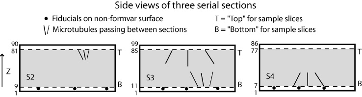
If you have N tomograms, then there are N-1 boundaries between sections. The words "top" and "bottom" are used here with a particular meaning: the "bottom" of a section is the part of the tomogram that will end up at lower Z in the final joined volume, while the "top" is the part that will end up at higher Z in the final volume. The "top" of one section thus matches up with the "bottom" of the next section higher in Z. These words do not refer to the high Z and low Z portions of a tomogram, so the top of a section may be at either the high or the low Z end. Indeed, if you invert the order in which the tomograms are to be stacked from low to high Z, you will change which side of each tomogram is considered the top by this definition. The programs will take care of any inversions in Z, both in extracting sample slices and in assembling the final volume, so you do not need to worry about entering slice numbers in a particular order.
If you have numbered your sections in the same order as they came off of the block during cutting, then the surface of a section against the formvar should be the top, and the other surface should be the bottom. You should be able to distinguish these surfaces by which one has gold particles closest to the sectioned material.
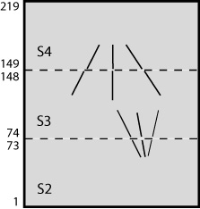
The following figures illustrate the meaning of these terms and how they translate into slice numbers to place in Etomo's table, for a case where all the sections have a consistent orientation. Refer back to these figures as you read through the more detailed instructions below.
The order in which you stack the sections will determine whether the handedness of structures is preserved or inverted from the individual tomograms to the joined volume. When the final joined volume is made, slices are stacked in either original or inverted Z order, and in the latter case handedness is inverted. When you finish the setup process, Etomo will signal to you whether tomograms are being inverted. If you care about handedness, the points to remember are:
The interface in Etomo was designed to work only with tomograms that have been flipped or rotated after generation so that the Z sections in the image file correspond to actual slices in Z, parallel to the plane of section. If you identify a tomogram for joining that appears not to have been flipped in the post-processing step, Etomo will offer to flip it for you and produce a file with extension ".flip" in the working directory. However, this will invert the handedness of structures in the volume.
To begin joining tomograms, start Etomo and select New Join from the File menu. This will bring up the Setup panel.
After opening the Setup panel, you must first make an entry for Working directory. You should create a new directory for your joining operation so that it is easy to clean up afterwards. You do not need to copy the tomograms into this directory. You can use the file chooser to browse for the directory, as well as to make a new folder and rename it to the desired name.
You must also enter a Root name for output file. The final tomogram will be named with this root name plus the extension ".join". An addition, a host of intermediate files will be created with this root name and other extensions. Files will be referred to below as, for example, "rootname.join". In addition, Etomo will automatically save a file, "rootname.ejf", to the working directory with all of its information about the joining operation. You can exit Etomo and restart where you left off by loading this file.
Press Add Section to add a section to the table, then use the file chooser to find the tomogram. The program will record the full path to the file but show only the file name. You can press the > button in the title line of the table to switch back and forth between seeing the full path and just the file name.
Once you have added a section, you need to select the section to perform any operations on it. This is done with the => button to the left of the file name.
You can change the order of the sections in the table by selecting a section and using Move Section Up or Move Section Down. You can also delete a section if necessary.
Once you have selected a section, you can view it in 3dmod by pressing Open in/Raise 3dmod. Note that you can bin the images in X and Y to reduce the amount of memory that they will require; this option should allow you to view several sections at once regardless of how big they are. Binning is only in X and Y, not in Z, so that slice numbers will not vary with binning.
It is possible to rotate a tomogram before joining, using Rotatevol. There are three reasons to use rotations.
Rotations should be avoided unless they are necessary for one of these reasons, not only to save time and disk space, but also to avoid degrading the images by multiple transformations. Thus, if you need to rotate for the second reason given above, rotate by exactly 90 degrees rather than by the angle that aligns the sections best, since the rotation will then not require any interpolations. Similarly, if you need to turn a volume upside down, rotate by 180 degrees unless a different angle is needed to correct a pitch in the reconstruction.
If you want to use Rotatevol to adjust the orientation of a section, then load the tomogram into 3dmod. Open a Slicer window and adjust the angles to achieve the desired rotation. It may take only a few tenths of a degree to correct significant pitch in the section. Use the numeric keypad arrow keys to adjust an angle by small increments (4 and 6 for 0.1 degree increments, 2 and 8 for 0.5 degree increments). Once you have obtained the desired rotation, be sure the section in question is selected in the section table, and press Get angles from slicer in Etomo to get the angles entered into the table.
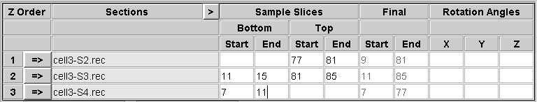
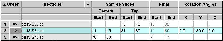
You need to decide which slices to extract from the top and bottom of each section in order to construct a file that contains a sample of each boundary. You should include the last slice that contains usable image data, and 5 to 10 slices into the section from there. This will allow you to see if there are trends in position within the section that need to be taken into account when aligning across the boundary. In some cases, this may not be needed, and you could choose to extract just one slice that is adequate for alignment. In general, it is safer to be generous in this initial sample. These sample slices will also be averaged to produce images that can be used for automatic alignment. Enter the first and last section of each range in the appropriate text box under Start and End, respectively, in the Sample Slices area of the table.
Note that the bottom of the first section and the top of the last section will not be extracted because they do not connect to another section.
At the same time that you are making these choices, you may also be able to decide what range of slices from each tomogram to include in the final volume. Enter these choices in the text boxes in the Final area of the table. These entries will appear in italics to signify that they are not relevant to the operation performed on this panel. Note that if you are rotating a section, these slice numbers picked in the original volume will be converted to the appropriate slices in the rotated volume, and the converted slice numbers will appear when you get to the Join panel.
When the sample slices are extracted, they will be transformed if necessary so that they are no bigger than a certain size. This size is 1024 pixels by default, but if your volumes are very large in X or Y this default may lose too much detail. To change the default, enter a larger number in the Squeeze samples to text box.
The combining procedures will scale the densities of the different sections to match their means and standard deviations. The same scaling will be applied in producing both the sample slices and the final volume. By default, the first section will be used as the reference for this scaling. If this section has poor dynamic range (i.e., black and white sliders need to be set close to each other in 3dmod to get good contrast), then all of the other sections will be scaled to a similarly poor dynamic range. To avoid this, select a different section as the reference using the Reference section for density matching entry.
When all entries have been made, press Make Samples. The program will first determine the density scaling. It will then run Rotatevol on any sections that have rotation angles, producing a file with extension ".rot" in the working directory. Finally, it will extract the sample slices into "rootname.sample" and average them into "rootname.sampavg". At this point, you can go on to the Align panel.
After you have made samples, most fields on the Setup panel will be disabled, to prevent disagreements between the information on this panel and the information used in later phases of the process. If you want to make new samples with different entries, just press Change Setup. After doing this, you are free to rearrange sections and modify entries, but you will not be able to go on to the other panels until you have made samples again. If you change your mind and just want to go on, press Revert to Last Setup to restore the entries that were used to make the existing samples. This will unlock the other tabs.
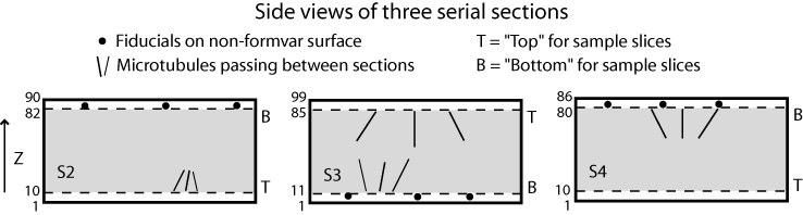
After you run Make Samples, Etomo is able to calculate whether some or all of the sections will be inverted in the final join. It will highlight inverted sections with yellow in the table and warn you if morethan half are being inverted. At this point, you can press Change Setup then Invert Table to invert the order of sections and change the inversion, if this will give the desired result. The program will manage all of the starting and ending slice entries, so you can just go on and make new samples.
The following figures show a more complicated example illustrating rotations and inversions. If the sections were stacked in this order, the resulting joined volume would be identical to the one shown above. However, in this case that stacking would invert the handedness, so this is a case where inverting the table would be helpful.
The Align panel has three components. There is a modified version of the section table with information relevant to aligning the sections; an area for setting parameters for automatic alignment, and buttons to perform the different kinds of alignment.
Midas can be used exclusively to align the sections manually, or it can be used to check and refine the results from automatic alignment. The sample slices are aligned in Midas using a special "chunk" alignment mode, in which you can adjust the alignment between chunks of slices while viewing any pair of slices from the chunks. For each section boundary, it will initially show the slice from the top of the lower section as the Reference sec. and the slice from the bottom of the upper section as the Current sec.. However, you are free to select another pair of slices for aligning, to scroll through either set of slices to assess trends in the structures, and to switch the pair of slices after you have started aligning. Use the up and down arrows on the spin boxes, or the "a", "b", "c", and "d" hot keys to move forward and back through the slices in the two sections. Use the "Current chunk" spin box or the "A" and "B" hot keys to switch to a different section boundary. If you get confused after stepping between slices, consult the right side of the section table, which shows the range of slices that can validly be used as reference and current sections for a given current chunk.
In Midas, you can also align slices with a nonlinear transform, i.e., warping, if the linear transformation is inadequate. Essentially, after aligning as much you wish with a linear transformation, you select the option to add warping points. You then add a series of points at locations where there are features that can be aligned. At each location, you shift the image locally into alignment. See the section Warping Images in the Midas man page for more details. Note that you can also use the warping functionality with just three points as an alternative way to stretch an image, and you still have a linear transformation.
Once you have introduced warping, the programs for transforming images and models will work with warping transforms instead of linear transforms. You can reopen Midas with the warping transforms and adjust. However, you cannot use Refine Auto Alignment to refine the alignment automatically once there are warping transforms.
In some cases, automatic alignment of the sample averages with Xfalign may produce an adequate alignment. The interface provides for using Xfalign in two different scenarios: getting an initial alignment that might need refinement by hand, or refining an approximate alignment that you have made with Midas.
By default, the automatic alignment will search for a full linear transformation, including translation, rotation, size change, and stretching. If the images do not contain enough information to indicate all of these aspects of a transformation, the search may be more successful if you restrict the transformation. You can select either Rotation/Translation/Magnification to omit stretch from the search, or Rotation/Translation to find an alignment that includes only rotation and translation. These are options to try before giving up on automatic alignment.
The filtering parameters control the degree of filtering that is applied to the images. The filtering is applied after the default image reduction by a factor of 2 in the program Xfsimplex, which searches for a transformation that minimizes a pixel-to-pixel difference between the images, summed over all pixels. This minimization is sensitive to noise, so some high-frequency filtering is appropriate. You might want to reduce the Cutoff for high-frequency filter below 0.35 for particularly noisy images.
The Join panel shows another variant on the data table in which you can adjust the starting and ending slices for the final volume. The panel also provides the ability to set the size and centering of the volume, to generate a trial volume quickly, and to adjust the size and centering with a rubber band in the trial volume.
At the top of the panel is an option to specify one of the sections as the reference to which the others will be aligned. By default, all tomograms will be transformed into alignment to a single average position. If you turn on Reference section for alignment and select a section, that section will not be transformed and the others will be. This is useful if you have already modeled on one section, or if you are adding another section to an existing set of serial sections. Note that if you have some sections that are rotated by large angles (90 or 180 degrees) relative to the rest, it is no longer necessary to set one section as a reference. The program Xftoxg will determine the most common orientation in the set of sections and compute the average alignment position from the sections at that orientation.
When you first enter the panel, it will show an output size that equals the maximum size of the input sections. If you have an appreciable shift between the sections, this size may not be sufficient. On the other hand, the area may be more than you need. The following procedure is recommended:
Once you have a joined volume, it is possible to model some of the features in the volume and use those features as fiducials for refining the alignment with Xfjointomo. The model can contain pairs of points that should correspond between two sections. It can also contain features such as oblique microtubules that are otherwise hard to use for alignment because their position shifts between the top of one section and the bottom of the next. If there are enough data from trajectories, it is even possible to determine the proper spacing between sections. See the Xfjointomo man page for complete details on how the program works.
You can still refine the alignment if you used warping for the initial alignment, but Xfjointomo will (thus far) solve only for a linear refining transformation. The final transformations applied in rejoining the volumes will still be warping transforms, since they are obtained by multiplying the initial warping transforms with the refining transforms. In order to build on the initial alignment as much as possible, the warping control points that you have already identified as corresponding between the sections are incorporated as fiducials in the refining model. Etomo takes care of this (as of IMOD 4.11) by running Joinwarp2model to initialize the refining model.
The fiducial model can be built on the final joined file, or a binned trial join file that includes all of the slices. The interface will not allow you to use a trial join that skips slices.
To start the refinement process, press the Refine Join button on the Join panel, which causes the program to rename the file that you want to model and store the information that it will need for the refinement. If you used warping in the initial alignment, this is the point at which Etomo runs Joinwarp2model.
Next, go to the Model tab and press Make Refining Model. Note that you can make this model on a binned or unbinned volume, just as you can make it on a binned trial join file. If you need to load the volume with binning, right-click on the Make Refining Model button to see the options for loading the volume binned by 2 and for opening 3dmod via the Startup dialog.
Here are the relevant points from the Xfjointomo man page on preparing the model:
Modeling trajectories: Data from trajectories such as microtubules are used to determine a pair of positions at a boundary between two sections, each position determined by extrapolating the trajectory on each side of the boundary. When you model trajectories such as microtubules, use enough points on each side of a boundary so that a line fit will give a reasonable extrapolation of the trajectory. The number of points used for the line fit is controlled by the values for the minimum and maximum number of points to fit; by default, fits will be done to 5 points if they are available, and to a minimum of 2 points. Thus, if a microtubule is curved at some distance from a boundary, you should add points densely enough so that the points being fit will be in a straight segment near the boundary. Avoid using the "Fill in Z" option, because that will create redundant data between actual points within a section, and incorrect data in a line segment across the boundary. If a feature being modeled crosses multiple section boundaries, you can model it all in one contour or start a new contour for each boundary.
Modeling pairs of points: Use contours with only two points in them to specify the centers of features that should align across a boundary. You may find that setting a symbol size or spherical point size for each point allows you to judge the centering of the point in a feature such as a vesicle. Pairs of points in such contours are included together with the pairs of positions extrapolated from trajectories in a single least-squares fit to find the transformation at a boundary.
After making and saving the model, you are ready to set the parameters for finding transformations. By default, the same parameters will be used for all section boundaries. However, if necessary, you can run Xfjointomo on a subset of the boundaries, then change the parameters and run on other boundaries. For example, if you run on all boundaries and get good results with some but not with others, you can change parameters and rerun only on the boundaries that gave poorer results. Each time the program runs, Etomo updates the Boundary Table only for the boundaries that were included and retains previous results for the others.
To set parameters for finding transformations:
Press Find Transformations. The Boundary Table will show the mean and maximum error of the fit over all points at a particular boundary. If you tried different gaps, the values shown will be at the gap that gave the lowest error. You can open the log file to see how the error varied with gap size. If the lowest error occurred at the first or last gap size, you might want to rerun with a larger range of gap sizes to be sure that is actually the size with the lowest error. On the other hand, if the variation of error with gap size is very slight, the determination of the best gap might be inaccurate and you might be better off constraining the gap to a smaller range or fixing it at zero.
Once you have a transformation for all boundaries, you can press Transform and View Model to see the fiducial model transformed into alignment. This can provide a quick check for whether kinks in the trajectories have been removed adequately, or whether some trajectories are problematic.
To join the tomograms with the refined alignment, go to the Rejoin panel. This panel allows you to adjust which slices will go into the new volume, make a trial or final rejoin, and transform any model file from the old alignment to the new one. On the upper left is a copy of the section table showing the starting and ending slices that went into the original final join. You can use the controls here to open one of the volumes and evaluate slices that are being added or dropped due to a change in spacing between sections.
On the upper right is a Boundary Table; for each boundary it shows the ending slice taken from the top of the section below, and the starting slice taken from the bottom of the section above. If a best gap was determined, then these slice numbers will be modified to create a gap of the given size. The adjusted numbers are shown in the right two columns. You can change any of these numbers with the spinners; if you do, the program will change the adjacent number so as to maintain the same spacing between sections. If you or the program selects a slice number beyond the range of the section (less than 1 or greater than the number of slices in the section), then blank slices will be inserted corresponding to the number of slices outside the actual section.
The remaining sections of the Rejoin panel are straightforward: