Join Tutorial

Tutorial for Joining Serial Section Tomograms with Etomo
(IMOD Version 4.9)

Cindi L. Schwartz

University of Colorado, Boulder

I. Initial steps

This tutorial provides a step-by-step guide to joining together tomograms from serial sections, using a small sample data set containing three volumes to be joined. Before you try to join your own tomograms, please refer to the more comprehensive Guide to Joining Tomograms for additional detail about the decisions and options at each step.

To get started, download the sample data set from our web site. Unpack the data by typing:

imoduntar joinTutorialData.tar.gz

This will create a directory, joinTutorialData, containing the three serial volumes, named basal-1.rec, basal-2.rec, and basal-3.rec.

II. Etomo Setup

To start Etomo, at the command line type: etomo

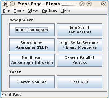
This will load the Etomo's Front Page. To get to the join setup page press the Join Serial Tomograms button.

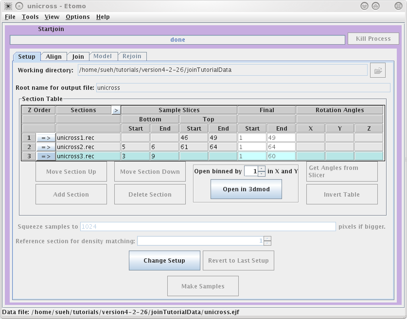
This will load the Join Interface shown below. The interface is divided into five panels: Setup, Align, Join, Model, and Rejoin. The Setup panel allows you to identify which serial tomograms you would like to join, define the surfaces at which they should be joined, flip or rotate the volumes relative to each other, and extract sample slices from each serial tomogram so that you can visualize the boundaries between the serial tomograms and align them. You will notice that you cannot use the Align or Join tabs until you have finished filling in the Setup information and make your sample file.

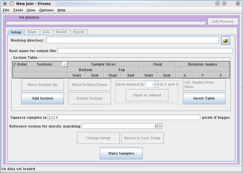
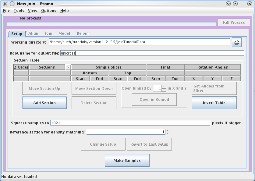
To get started, select your Working directory and Root name for output file. In this example, we used a directory called JoinTutorialData and used unicross for the root name. You can enter the Working directory by clicking on the yellow file selection button associated with the Working directory field, or by typing in the directory path and file name directly in the field. Since you already have all of the individual reconstructions in the joinTutorialData directory, your can make that be your working directory.

Next, you need to select the serial tomograms you want to join by pressing the Add Section button. It will take you to your Working directory and allow you to select a file for joining. (Note that you are not required to put your serial tomograms in your working directory. Etomo will keep track of where your files are located). You must add each serial tomogram individually. The initial order is not important because you can change the order later.

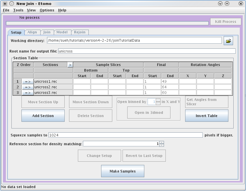
Once you have input all three datasets, click on the arrow in the Z Order subsection to highlight unicross1.rec. Now click on the Open in 3dmod button. This will open unicross1.rec using 3dmod. These tutorial datasets are small in size; however, for future data, you may need to use the binning option to view all of your serial tomograms at once. Now, open the other two serial tomograms with the Open in 3dmod button. Once all three tomograms are loaded, you will typically movie through them to figure out the order of the serial tomograms and what slices you would like to use to create the samples that are used in the aligning process. It is important to note that Bottom and Top are used in the join software to denote that the 'top' of the section is the part of the tomogram that matches up with the 'bottom' of the next section. 'Top' and 'bottom' DO NOT refer to the high Z and low Z portions of the tomogram. So, the top of a section can be at either high or low Z. The join programs will take care of any inversions in Z, both in extracting sample slices and in assembling the final volume. The 'Bottom' entry in the first row and the 'Top' entry in the last row are not necessary because they don't match up to another tomogram. To determine the Sample Slices you need, see the entries we have used below. The goal here is to find a small subsection of the ends of each serial tomogram that you can use to align. Note that the Bottom of unicross2.rec starts at Z= 5. This is becausethe gold on the surface does not give you any information to align with, so you need to go deeper into the tomogram. You can also select the slices that represent the Final Start and Final End of each tomogram now, but you will get a chance to change this later on in the Join tab. These numbers determine which slices will be placed into the final joined volume.

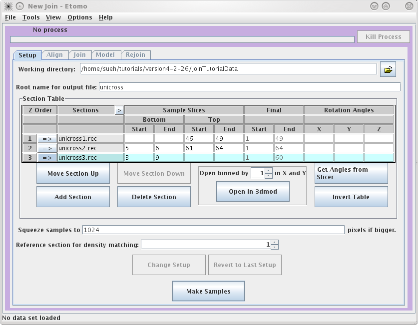
Once you are satisfied with your decisions, press the Make Samples button. This creates unicross.sample which will be used in conjunction with Midas to visually align the serial tomograms together. After unicross.sample is created, you can now access the Align and Join tabs. You will notice that you can always come back and use Change Setup to pick new Sample Slices and start over.

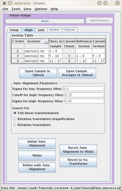
III. Aligning the Sample Slices

The Align tab allows you to align the serial tomograms before joining them together. It is a good idea to Open Sample Averages in 3dmod. By toggling through Z, you can see whether you have chosen the correct Sample Slices. For instance, toggle between Z=1 and Z=2. You can see these are a close match by looking at the cluster of vesicles in the lower right corner, but they are not aligned to each other. Now you can choose to try auto alignment or manual alignment of the serial tomograms. These tutorial tomograms lend themselves well to auto alignment. Click on Initial Auto Alignment and wait for done to appear in the process bar. Now, click on Midas. 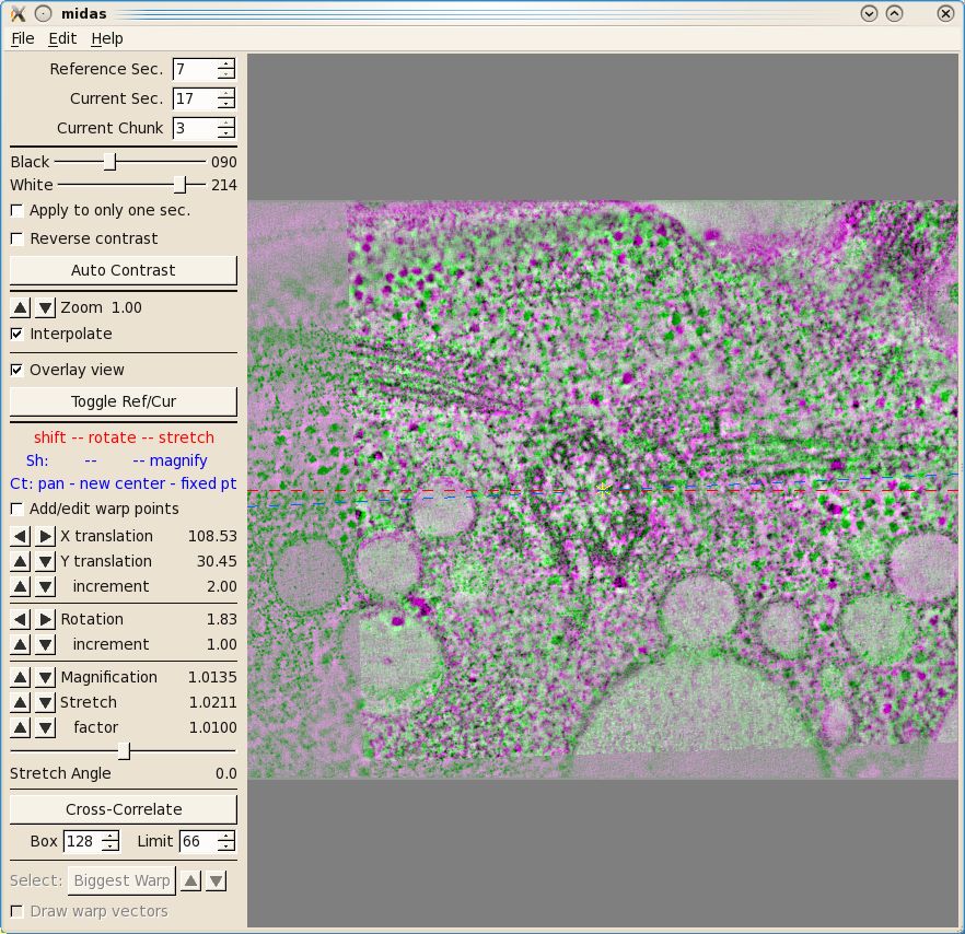This will load the program midas which allows you to see how well the auto alignment worked.

The first thing you will see inMidas is an overlay view showing contrasting magenta and green colors that help you align images. What is first displayed is the 'top' of unicross1.rec aligned with the 'bottom' of unicross2.rec. Midas considers each tomogram as a single 'chunk' of slices, so it is actually showing the alignment of the bottom of 'chunk 2' to the top of 'chunk 1'. You can use the Toggle Ref/Cur button to see the alignment better by toggling between the images, and the PageUp and PageDown keys can also be used to see one image at a time. If the sample slices being displayed do not have a clear image of the structures at the surface of the volume, then you can step deeper into either section by reducing the Reference Sec. number or increasing the Current Sec. number. The Reference Section remains fixed and the Current Section is shifted relative to this to align the two images. Midas lets you shift, rotate, or stretch the Current Section with the left, middle, and right mouse buttons, respectively. Alternatively, the arrow buttons on the left panel in Midas will perform the same functions. To advance to the next alignment pair, make the Current Chunk 3 to align the next pair of tomograms.

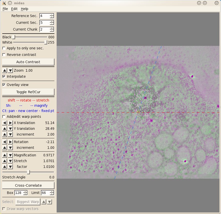
Now you see the 'top' of unicross2.rec aligned with the 'bottom' of unicross3.rec. You can also try and manually improve this alignment. If you make changes you want to keep, be sure to save them under File-Save Transforms.

If you make changes and realize that they aren't as good as the auto alignment, you can always use the Revert to No Transforms button and start over.

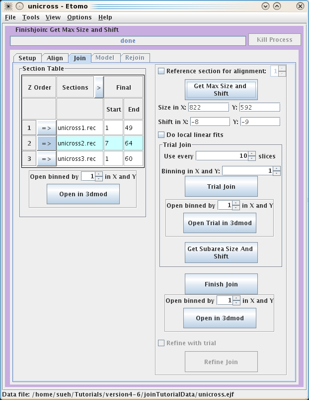
IV. Joining the Serial Tomograms

Once you are happy with the alignments, you can now move to the Join tab. First, you can pick the starting and ending slices of each serial tomogram you would like to keep for the final volume if you did not enter these in the Setup page. Again, you are given the option to view each tomogram by using the Open in 3dmod button. These serial tomograms provide an example where using the Get Max Size and Shift button can be useful. The program will calculate the Size and Shift in X and Y required to keep all original data in the final volume and automatically put the numbers in the proper fields. Now you can use the Trial Join button to get a very quick idea of what your final volume will look like. This is very useful with larger datasets because the join process can take a long time. Once the Trial Join is finished, Open Trial in 3dmod to view it. The Get Subarea Size And Shift button is used if you wish to crop the final volume to a particular area with the rubberband feature in 3dmod. If you are happy with your Trial Join, click Finish Join to create your final volume. This could take a long time depending on the size of your original datasets. Once the program has finished, use Open in 3dmod to see your final volume called basal.join. Again, there is no need to use the binning feature with these data, but it will likely be necessary for real datasets. Often, it is necessary to improve the alignment of the serial section join using a refining model described in the following section.

V. Making a fiducial model to improve the alignment of serial tomograms

Creating the fiducial model

If the alignment from the previous step needs further refinement, this can be done using the series of steps described in this section. After finishjoin has created the serial section join, the Refine Join button will become available. Press this button and then proceed to the Model tab. The goal of creating a refine model is to identify a set of corresponding features that span across the serial tomograms and to model and use these features as alignment markers to improve the alignment. The fiducial model can be built o the final joined file or a binned trial join file that contains all of the slices. In the following example, microtubles and vesicles (or membrane compartments) are used to create the fiducial model. Press the Refine Model button to open the joined tomogram in 3dmod. This will also open a model that has one object assigned as an open countour object.

Micotubules are useful alignment features that span as trajectories between serial tomograms. Data from trajectories, such as microtubules, are used to determine a pair of positions at a boundary between two sections, each position determined by extrapolating the trajectory on each side of the boundary. 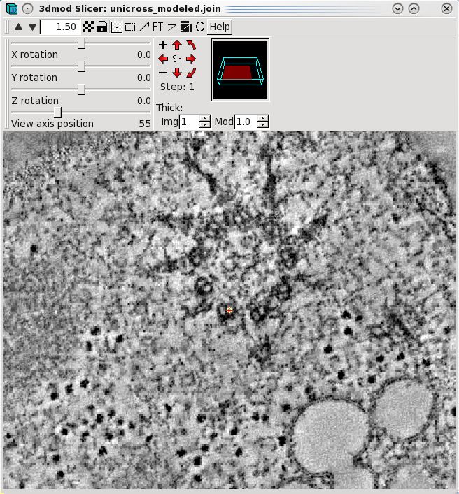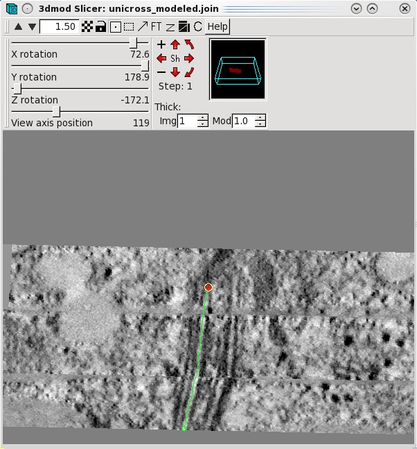It is important to use enough points on each side of the boundary so that the trajectory can be extrapolated appropriately. It is useful to use the slicer window to model microtubule trajectories across the serial tomogram boundaries. Open the slicer window by hitting the \ hot key or select Image-Slicer from the 3dmod main menu. The window on the left shows a basal body cross section in the slicer window. Highlight the middle of a microtubule using the left mouse button. Rotate the x,y and z sliders so that the microtubule appears in longitudinal view. In this example, the sliders were adjusted to 72.6, 178.9 and -172.1, respectively. Place model points along the length of the microtuble using the middle mouse button as shown by the green line. Create a new contour for each new microtubule.

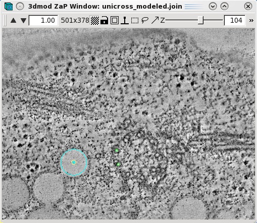
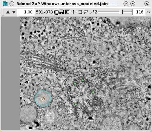
Features, such as vesicles, can also be modeled as pairs of points to specifiy the centers of the object that should align across a boundary. Create a new object by selecting Edit-Object-New and assign the object type as a scattered point object. Adjust the spherical point size so that the diameter of the sphere fits the vesicle. Place one model point in the center of the vesicle on one boundary and one point in the center of the vesicle on the other boundary. In the example below, the boundaries of the serial tomogram were on sections 104 and 116, respectively. Make a new contour for each new vesicle. Save the model after modeling a number of features that span the serial section boundaries.

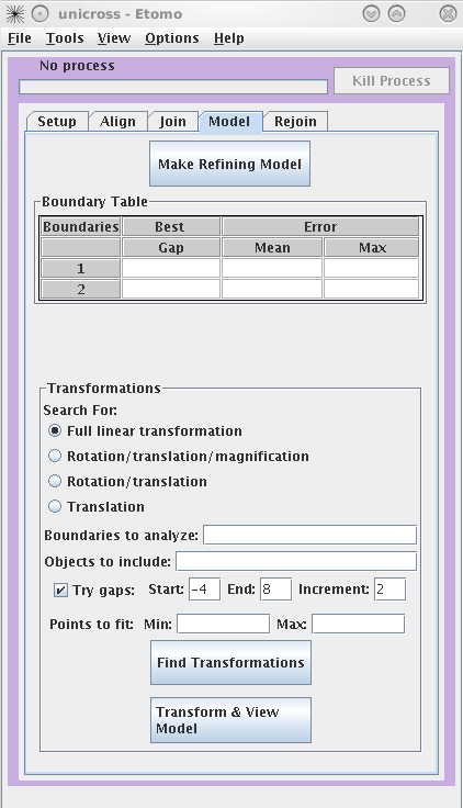
Finding transformations

By default, a full linear transformation using all model objects and all boundaries is selected. This is appropriate as long as you have at least 6 features well-distributed over the whole area. Otherwise, you should select a more restricted transformation with the radio buttons. Searching for the best gap between sections is also selected by default, and should be used if there are some oblique trajectories (ones that do not run perpendicularly through the sections). Otherwise, you should uncheck Try gaps. Hit the Find Transformations button. The Boundary Table will update with the mean and maximum error of the fit over all points at a particular boundary. The table will also report the best gap to adjust the spacing between tomograms for the best fit.

Press the Transform & View Model to see the fiducial model transformed into alignment. If the aligned model looks smooth (the trajectories are not kinked), proceed to the Rejoin tab to join the tomograms with the refined alignment.

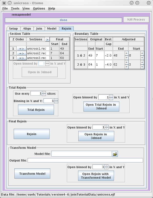
Rejoining with Refining Transforms

The Rejoin panel contains a Section Table to adjust which slices will go into the new volume. The Boundary Table reports the adjusted section slices if gaps were found.

A Trial Rejoin of the joined tomogram can be run using the adjusted start and end values and the Trial Rejoin can be opened in 3dmod. If you are happy with the alignment press Rejoin to apply the refined alignment to all slices. Open Rejoin in 3dmod to view the final, joined tomogram. Transform Model can be used to transform the fiducial model used for refining so it fits on the final, joined tomogram, or it can be used to transform any other model built on the original joined tomogram. Select the Model File, specify an Output file name and then press Transform Model. Finally, press Open Rejoin with Transformed Model to view the final, joined tomogram with the realigned model.